IPW analysis of nested case-control data

The classical nested case-control (NCC) analysis conditions on the sampled risk sets: each case and its matched controls form a stratum, and estimator = "clogit" uses the conditional partial likelihood (see vignette("nested-cc")). Controls appear only at their matched case’s failure time — a design feature that removes residual confounding by the matching variables but also discards information each control carries across the full follow-up.

The inverse probability weighting (IPW) approach breaks the matching. Each sampled control receives a weight equal to the inverse of its inclusion probability under the NCC sampling scheme, then a standard weighted Cox partial likelihood is fit over the unique subjects (cases + unique controls). Controls now contribute at every event time where they are still at risk — their exposure information is re-used across all failure times rather than only at their matched event. This gains efficiency, especially when many controls were matched to early cases and their follow-up extends across later events.

Code

library(matchatr)

Generating a cohort and an NCC sample

Code

set.seed(77)
n      <- 3000
beta_x <- log(2)                       # true Cox log hazard ratio
exposure   <- rbinom(n, 1, 0.4)
confounder <- rnorm(n)
rate       <- 0.08 * exp(beta_x * exposure + 0.4 * confounder)
tt         <- rexp(n, rate)            # single draw for consistent t and d
cohort <- data.frame(
  id         = seq_len(n),
  t          = pmin(tt, 5),
  d          = as.integer(tt <= 5),
  exposure   = exposure,
  confounder = confounder
)

sample_ncc() with incl_prob = TRUE draws the NCC sample and appends two columns needed for the IPW analysis:

ipw_weight — the Samuelsen (1997) inverse inclusion probability 1/π_j for each sampled control; cases get weight 1. The inclusion probability is the Kaplan-Meier-type formula π_j = 1 − prod of (1 − m_i / n_elig_i) over all event times where j was eligible, where m_i is the controls sampled and n_elig_i the eligible pool size.
.cohort_row — original cohort row index, used to deduplicate controls that were sampled into multiple risk sets before fitting the Cox model.

Code

set.seed(1)
ncc <- sample_ncc(cohort, time = "t", event = "d", m = 3, incl_prob = TRUE)
ncc[1:6, c("id", "t", "d", "exposure", "case", "set", "risk_time",
           "ipw_weight", ".cohort_row")]
#>       id           t     d exposure  case   set   risk_time ipw_weight
#>    <int>       <num> <int>    <int> <int> <int>       <num>      <num>
#> 1:  1449 0.001839354     1        0     1     1 0.001839354   1.000000
#> 2:  1017 5.000000000     0        0     0     1 0.001839354   1.243534
#> 3:   679 5.000000000     0        0     0     1 0.001839354   1.243534
#> 4:  2178 5.000000000     0        0     0     1 0.001839354   1.243534
#> 5:  1124 0.019657203     1        0     1     2 0.019657203   1.000000
#> 6:   930 5.000000000     0        1     0     2 0.019657203   1.243534
#>    .cohort_row
#>          <int>
#> 1:        1449
#> 2:        1017
#> 3:         679
#> 4:        2178
#> 5:        1124
#> 6:         930

Fitting the IPW weighted Cox model

With estimator = "ipw_cox", matchatr:

Deduplicates the NCC data by .cohort_row (each cohort subject appears once in the analysis).
Fits coxph(Surv(t, d) ~ exposure + confounder, weights = ipw_weight, robust = TRUE).
Returns the Lin-Wei robust sandwich variance via coxph(robust = TRUE).

Code

fit_ipw <- matcha(
  ncc,
  outcome     = "d",          # cohort event indicator, not the per-set "case"
  exposure    = "exposure",
  design      = nested_cc(strata = "set", time = "t"),
  confounders = ~confounder,
  estimator   = "ipw_cox"
)
fit_ipw
#> <matchatr_fit>
#>  Design:     Nested case-control
#>  Estimator:  ipw_cox  (engine: ipw_cox)
#>  Outcome:    d
#>  Exposure:   exposure
#>  Confounders: ~confounder
#>  N:          5028  (cases: 2164, controls: 2864)

Code

contrast(fit_ipw)             # reports type = "hr" by default
#> <matchatr_result>
#>  Estimator:  ipw_cox  (engine: ipw_cox)
#>  Estimand:   hazard ratio
#>  Contrast:   Hazard ratio
#>  CI method:  model
#>  N:          2650
#> 
#> Contrasts:
#>    comparison estimate        se ci_lower ci_upper
#>        <char>    <num>     <num>    <num>    <num>
#> 1:   exposure 1.933088 0.1157639 1.719004 2.173833

Comparison: classical NCC vs IPW NCC vs full cohort

The conditional partial likelihood (clogit) and the IPW weighted Cox target the same hazard ratio; the IPW estimator is at least as efficient because it reuses controls across failure times.

Code

# Classical NCC (clogit, matched analysis) — same seed as the IPW sample above
set.seed(1)
ncc_classical <- sample_ncc(cohort, time = "t", event = "d", m = 3)
fit_clogit <- matcha(ncc_classical, "case", "exposure",
                     nested_cc(strata = "set", time = "t"),
                     confounders = ~confounder, estimator = "clogit")

# Full-cohort Cox (the gold standard)
fit_full <- survival::coxph(
  survival::Surv(t, d) ~ exposure + confounder, data = cohort
)

cat("Full-cohort Cox HR: ", round(exp(coef(fit_full)["exposure"]), 3), "\n")
#> Full-cohort Cox HR:  1.922
cat("Classical NCC HR:   ", round(contrast(fit_clogit)$contrasts$estimate, 3), "\n")
#> Classical NCC HR:    1.887
cat("IPW NCC HR:         ", round(contrast(fit_ipw)$contrasts$estimate, 3), "\n")
#> IPW NCC HR:          1.933

All three estimates target the same hazard ratio; the classical and IPW NCC estimates will differ by a small simulation noise term.

tidy() output

Code

tidy(contrast(fit_ipw))
#>        term estimate std.error   type conf.low conf.high
#>      <char>    <num>     <num> <char>    <num>     <num>
#> 1: exposure 1.933088 0.1157639     hr 1.719004  2.173833

Rejection paths

Code

# Requesting an odds ratio from an IPW NCC fit is rejected (wrong scale).
contrast(fit_ipw, type = "or")
#> Error in `contrast()`:
#> ! The IPW NCC weighted Cox estimator reports hazard ratios, not `type = "or"`.
#> ℹ Use `type = "hr"` (the default for `ipw_cox`).

Code

# Bootstrap is not available for the IPW Cox estimator.
contrast(fit_ipw, type = "hr", ci_method = "bootstrap")
#> Error in `contrast()`:
#> ! `ci_method = "bootstrap"` is not available for the IPW Cox estimator.
#> ℹ Use `ci_method = "model"` (the robust Lin-Wei interval from `coxph(robust = TRUE)`) or `ci_method = "sandwich"`.

Code

# The ipw_weight column is required; sample_ncc() without incl_prob = TRUE
# produces data that lacks it.
ncc_no_wts <- sample_ncc(cohort, "t", "d", m = 3)
matcha(ncc_no_wts, "case", "exposure",
       nested_cc(strata = "set", time = "t"),
       estimator = "ipw_cox")
#> Error in `require_ipw_ncc_columns()` at matchatr/R/ipw_cox.R:39:3:
#> ! The `ipw_cox` estimator requires an `ipw_weight` column in `data`.
#> ℹ Use `sample_ncc(..., incl_prob = TRUE)` to generate the Samuelsen KM inclusion weights before calling `matcha()`.

Working-model weights

Samuelsen KM weights are design-based: they depend only on the risk-set structure and are computed during sample_ncc(). An alternative is to fit a working model for the selection probability — a logistic regression (or GAM) of whether a subject was selected as a control, given its covariates and the event time. Working-model weights can be more efficient when the logistic model is close to the truth.

compute_ncc_weights() replaces the ipw_weight column with working-model estimates. It requires the full Phase-1 cohort to reconstruct who was eligible (but not selected) at each event time.

Code

# Replace KM weights with GLM working-model weights
ncc_glm <- compute_ncc_weights(
  ncc,
  cohort           = cohort,
  method           = "glm",
  selection_formula = ~ risk_time,   # default: time-only logistic model
  time             = "t"
)
ncc_glm[1:3, c("id", "case", "set", "ipw_weight")]
#>       id  case   set ipw_weight
#>    <int> <int> <int>      <num>
#> 1:  1449     1     1   1.000000
#> 2:  1017     0     1   1.243532
#> 3:   679     0     1   1.243532

Fit and compare:

Code

fit_glm <- matcha(
  ncc_glm,
  outcome     = "d",
  exposure    = "exposure",
  design      = nested_cc(strata = "set", time = "t"),
  confounders = ~confounder,
  estimator   = "ipw_cox"
)
cat("KM weights HR: ", round(contrast(fit_ipw)$contrasts$estimate, 3), "\n")
#> KM weights HR:  1.933
cat("GLM weights HR:", round(contrast(fit_glm)$contrasts$estimate, 3), "\n")
#> GLM weights HR: 1.933

Both KM and GLM weights target the same Cox hazard ratio; differences reflect the working-model vs design-based weight formulas.

A GAM can be used when the selection probability is non-linearly related to time:

Code

ncc_gam <- compute_ncc_weights(
  ncc,
  cohort           = cohort,
  method           = "gam",
  selection_formula = ~ s(risk_time),
  time             = "t"
)
fit_gam <- matcha(
  ncc_gam,
  outcome     = "d",
  exposure    = "exposure",
  design      = nested_cc(strata = "set", time = "t"),
  confounders = ~confounder,
  estimator   = "ipw_cox"
)
cat("GAM weights HR:", round(contrast(fit_gam)$contrasts$estimate, 3), "\n")
#> GAM weights HR: 1.933

The Phase-1 cohort is required: omitting it aborts with matchatr_missing_phase1.

Code

compute_ncc_weights(ncc, cohort = NULL, method = "glm", time = "t")
#> Error in `compute_ncc_weights()`:
#> ! Working-model weight `method = "glm"` requires the full Phase-1 cohort data.
#> ℹ Supply the original cohort as `cohort`. It must contain the `time` column and any covariates in `selection_formula`.

Absolute risk

Because the IPW reformulation builds a weighted pseudo-cohort, it recovers the cumulative baseline hazard — which the classical conditional partial likelihood conditions away. absolute_risk() turns the fitted weighted Cox into a cumulative incidence

\[F_x(t) = 1 - \exp\!\big(-\exp(\hat\beta^{\top} x)\,\hat\Lambda_0(t)\big),\]

where \(\hat\Lambda_0(t)\) is an inverse-probability-weighted Breslow cumulative baseline hazard over the deduplicated analysis sample: at each event time the at-risk denominator \(\sum_j w_j \exp(\hat\beta^{\top} x_j)\) upweights each control by \(1/\pi_j\) so it stands in for the unsampled cohort. Confidence intervals use the delta method on the complementary log-log scale.

Code

newdata <- data.frame(exposure = c(1, 0), confounder = c(0, 0))
ar <- absolute_risk(fit_ipw, newdata = newdata, times = c(1, 2, 3, 4))
ar
#> <matchatr_absolute_risk>
#>  Engine:     ipw_cox
#>  Method:     IPW
#>  CI method:  delta (log-log)
#>  Times:      4 evaluation times (1, 2, 3, 4)
#>  Patterns:   2 covariate patterns
#> 
#> Absolute risk estimates:
#>      row  time  estimate   ci_lower   ci_upper
#>    <int> <num>     <num>      <num>      <num>
#> 1:     1     1 0.1371473 0.11799719 0.15911488
#> 2:     1     2 0.2553437 0.22557048 0.28826433
#> 3:     1     3 0.3771901 0.33877772 0.41842855
#> 4:     1     4 0.4661829 0.42308660 0.51144304
#> 5:     2     1 0.0734698 0.06605153 0.08168416
#> 6:     2     2 0.1414573 0.13119292 0.15245217
#> 7:     2     3 0.2172580 0.20474294 0.23042173
#> 8:     2     4 0.2772665 0.26336477 0.29174737

The hand-rolled weighted Breslow agrees with survival::survfit on the same weighted Cox model to machine precision, so the point estimate is exact; the interval is conservative (the within-sample Nelson-Aalen baseline variance).

Code

est <- ar$estimates
exposed   <- est[est$row == 1, ]
unexposed <- est[est$row == 2, ]
plot(exposed$time, exposed$estimate, type = "b", pch = 19, col = "#c0392b",
     ylim = c(0, max(est$ci_upper)), xlab = "time", ylab = expression(hat(F)[x](t)),
     main = "IPW NCC cumulative incidence")
lines(unexposed$time, unexposed$estimate, type = "b", pch = 19, col = "#2980b9")
legend("topleft", c("exposed", "unexposed"), col = c("#c0392b", "#2980b9"),
       pch = 19, lty = 1, bty = "n")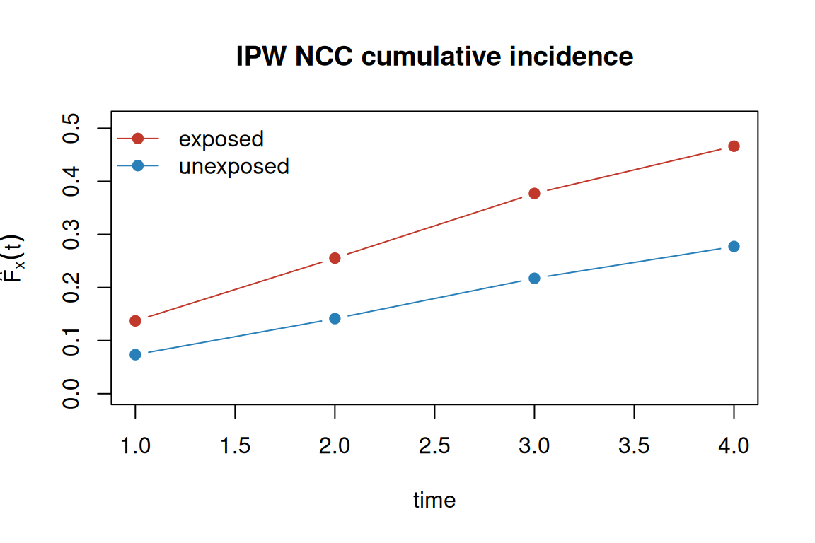

Cumulative incidence over follow-up for an exposed versus an unexposed subject estimated from the IPW nested case-control weighted Cox model. The exposed curve rises faster, reflecting the hazard ratio above one.

The same verb serves the case-cohort cch engine (see vignette("case-cohort")); only the baseline-hazard weighting differs.

Multiple endpoints from one control set

The real payoff of breaking the matching is control reuse across endpoints (Saarela et al. 2008). The classical conditional analysis ties each control to its case’s failure time, so a control set sampled for one endpoint cannot serve another. Under IPW the sample is a weighted pseudo-cohort, so the same controls can fit a weighted Cox for any endpoint recorded in the cohort. matchatr supports two modes.

We build a cohort with two competing endpoints — a harmful exposure for endpoint 1, a protective one for endpoint 2:

Code

set.seed(20)
n <- 4000
x <- rbinom(n, 1, 0.4)
z <- rnorm(n)
t1 <- rexp(n, 0.05 * exp(log(2.0) * x + 0.3 * z))   # endpoint 1: HR 2.0
t2 <- rexp(n, 0.05 * exp(log(0.5) * x + 0.2 * z))   # endpoint 2: HR 0.5
tau <- 6
tt    <- pmin(t1, t2, tau)
cause <- ifelse(tt >= tau, 0L, ifelse(t1 < t2, 1L, 2L))
co <- data.frame(
  id = seq_len(n), t = tt,
  d_any = as.integer(cause != 0L),   # any failure
  d1    = as.integer(cause == 1L),   # endpoint 1
  d2    = as.integer(cause == 2L),   # endpoint 2
  x = x, z = z
)

Mode A — sample on the union event, analyse each endpoint

Sampling on the “any-failure” event ascertains every endpoint’s cases at once, so each cause-specific endpoint is analysed directly by passing it as outcome. The single sampled control set, with its shared inclusion weights, backs both fits:

Code

set.seed(1)
ncc_multi <- sample_ncc(co, time = "t", event = "d_any", m = 3, incl_prob = TRUE)

fit_e1 <- matcha(ncc_multi, outcome = "d1", exposure = "x",
                 design = nested_cc(strata = "set", time = "t"),
                 confounders = ~ z, estimator = "ipw_cox")
fit_e2 <- matcha(ncc_multi, outcome = "d2", exposure = "x",
                 design = nested_cc(strata = "set", time = "t"),
                 confounders = ~ z, estimator = "ipw_cox")

rbind(cbind(endpoint = "d1", tidy(contrast(fit_e1))),
      cbind(endpoint = "d2", tidy(contrast(fit_e2))))
#>    endpoint   term  estimate  std.error   type  conf.low conf.high
#>      <char> <char>     <num>      <num> <char>     <num>     <num>
#> 1:       d1      x 2.1554205 0.12710968     hr 1.9201487 2.4195196
#> 2:       d2      x 0.4508881 0.04171509     hr 0.3761124 0.5405301

Both hazard ratios sit near their cohort truths (2.0 and 0.5). A competing-endpoint case is ascertained by the sampling, so it keeps weight 1 (not the control weight 1/π_j) when a different endpoint is analysed — matchatr handles this when it builds the deduplicated analysis sample.

Mode B — reuse a primary-endpoint control set for a secondary endpoint

If the NCC was drawn for a single primary endpoint, its controls can still be reused for a secondary one (Støer and Samuelsen 2012). reuse_ncc_endpoint() keeps the controls’ primary inclusion weights 1/π_j (the inclusion probability is a property of the sampling, not the endpoint) and augments the secondary endpoint’s cases that were not sampled — pulled from the Phase-1 cohort with weight 1, since every case of an analysed endpoint is ascertained with probability 1:

Code

set.seed(1)
ncc_primary <- sample_ncc(co, time = "t", event = "d1", m = 3, incl_prob = TRUE)

ncc_reuse <- reuse_ncc_endpoint(ncc_primary, cohort = co, time = "t", event = "d2")
fit_reuse <- matcha(ncc_reuse, outcome = "d2", exposure = "x",
                    design = nested_cc(strata = "set", time = "t"),
                    confounders = ~ z, estimator = "ipw_cox")
tidy(contrast(fit_reuse))
#>      term estimate  std.error   type  conf.low conf.high
#>    <char>    <num>      <num> <char>     <num>     <num>
#> 1:      x 0.458899 0.04307734     hr 0.3817806  0.551595

Reusing the secondary endpoint needs the cohort to recover its unsampled cases; omitting it is rejected:

Code

reuse_ncc_endpoint(ncc_primary, cohort = NULL, time = "t", event = "d2")
#> Error in `reuse_ncc_endpoint()`:
#> ! Reusing a control set for a second endpoint requires the full Phase-1 cohort.
#> ℹ Supply the original cohort as `cohort` so the secondary endpoint's cases that were not sampled can be ascertained.

Alternative models: time ratios and excess hazards

Breaking the matching also frees the analysis from the proportional-hazards scale. The same Samuelsen-weighted sample supports two non-Cox models, each reporting a different effect measure.

The accelerated failure time model (estimator = "ipw_aft") acts on the survival-time scale: contrast(type = "af") reports the time ratio exp(β) — the factor by which a unit of exposure multiplies the survival time (above one prolongs, below one shortens). It is a weighted Weibull survreg with a robust sandwich (Kang et al. 2017).

Code

fit_aft <- matcha(ncc, outcome = "d", exposure = "exposure",
                  design = nested_cc(strata = "set", time = "t"),
                  confounders = ~ confounder, estimator = "ipw_aft")
contrast(fit_aft)
#> <matchatr_result>
#>  Estimator:  ipw_aft  (engine: ipw_aft)
#>  Estimand:   time ratio
#>  Contrast:   af
#>  CI method:  model
#>  N:          2650
#> 
#> Contrasts:
#>    comparison  estimate         se  ci_lower  ci_upper
#>        <char>     <num>      <num>     <num>     <num>
#> 1:   exposure 0.5335832 0.03098763 0.4761776 0.5979093

The fitted Weibull is a full survival curve, so absolute_risk() also serves the ipw_aft engine — reading the cumulative incidence straight off the parameters, with no Breslow step:

\[F_x(t) = 1 - \exp\!\big(-\exp((\log t - \hat\eta)/\hat\sigma)\big),\]

where \(\hat\eta = \hat\beta^{\top} x\) is the AFT linear predictor and \(\hat\sigma\) the scale. The interval again uses the delta method on the complementary log-log scale, here over \((\beta, \log\sigma)\) with the robust survreg sandwich. Because the curve is parametric, \(\hat F_x(t)\) is smooth in \(t\) (the Cox engine’s \(\hat F_x(t)\) is a step function on the event times).

Code

ar_aft <- absolute_risk(fit_aft, newdata = newdata, times = c(1, 2, 3, 4))
ar_aft
#> <matchatr_absolute_risk>
#>  Engine:     ipw_aft
#>  Method:     IPW AFT (weibull)
#>  CI method:  delta (log-log)
#>  Times:      4 evaluation times (1, 2, 3, 4)
#>  Patterns:   2 covariate patterns
#> 
#> Absolute risk estimates:
#>      row  time   estimate   ci_lower   ci_upper
#>    <int> <num>      <num>      <num>      <num>
#> 1:     1     1 0.13304685 0.12027050 0.14706343
#> 2:     1     2 0.25649465 0.23727818 0.27696719
#> 3:     1     3 0.36514831 0.34124399 0.39018443
#> 4:     1     4 0.45949897 0.43196896 0.48793413
#> 5:     2     1 0.07100399 0.06359155 0.07924329
#> 6:     2     2 0.14177844 0.12993618 0.15460098
#> 7:     2     3 0.20894862 0.19337684 0.22559038
#> 8:     2     4 0.27195548 0.25295836 0.29208196

The baseline defaults to Weibull, but dist selects any of four AFT distributions — "weibull", "exponential", "lognormal", "loglogistic". All report the same time ratio exp(β); they differ in the survival-curve shape ("lognormal" / "loglogistic" allow a non-monotone hazard). absolute_risk() follows the chosen baseline automatically:

Code

fit_ln <- matcha(ncc, outcome = "d", exposure = "exposure",
                 design = nested_cc(strata = "set", time = "t"),
                 confounders = ~ confounder, estimator = "ipw_aft",
                 dist = "lognormal")
contrast(fit_ln)
#> <matchatr_result>
#>  Estimator:  ipw_aft  (engine: ipw_aft)
#>  Estimand:   time ratio
#>  Contrast:   af
#>  CI method:  model
#>  N:          2650
#> 
#> Contrasts:
#>    comparison  estimate         se ci_lower  ci_upper
#>        <char>     <num>      <num>    <num>     <num>
#> 1:   exposure 0.4990467 0.03379107 0.437024 0.5698717

The additive-hazards model (estimator = "ipw_aalen") acts on the rate scale: it writes the hazard as a sum, λ(t) = λ₀(t) + γ·exposure, so contrast(type = "excess") reports the excess hazard γ — an additive rate difference (Borgan and Langholz 1997). Unlike a ratio it can be negative (a protective exposure lowers the rate), and its confidence interval is symmetric (it is not exponentiated).

Code

fit_add <- matcha(ncc, outcome = "d", exposure = "exposure",
                  design = nested_cc(strata = "set", time = "t"),
                  confounders = ~ confounder, estimator = "ipw_aalen")
contrast(fit_add)
#> <matchatr_result>
#>  Estimator:  ipw_aalen  (engine: ipw_aalen)
#>  Estimand:   excess hazard
#>  Contrast:   excess
#>  CI method:  model
#>  N:          2650
#> 
#> Contrasts:
#>    comparison   estimate          se   ci_lower   ci_upper
#>        <char>      <num>       <num>      <num>      <num>
#> 1:   exposure 0.07596765 0.007473284 0.06132028 0.09061501

contrast() reports a single time-constant excess hazard (the Lin-Ying model; Lin and Ying (1994)). To let the effect vary with time, excess_risk() returns the cumulative excess hazard \(B_j(t) = \int_0^t \beta_j(s)\,ds\) — the additive analogue of absolute_risk(). A straight line means a constant rate difference; curvature means a time-varying one.

Code

er <- excess_risk(fit_add, times = 1:5)
er
#> <matchatr_excess_risk>
#>  Engine:     ipw_aalen
#>  Estimand:   cumulative excess hazard B_j(t)
#>  CI method:  Aalen martingale
#>  Times:      5 evaluation times
#>  Terms:      exposure, confounder
#> 
#> Cumulative excess hazard:
#>           term  time   estimate         se   ci_lower   ci_upper
#>         <char> <int>      <num>      <num>      <num>      <num>
#>  1:   exposure     1 0.07098524 0.01384925 0.04384121 0.09812927
#>  2:   exposure     2 0.15270345 0.02027272 0.11296965 0.19243724
#>  3:   exposure     3 0.25131671 0.02676949 0.19884948 0.30378394
#>  4:   exposure     4 0.31075495 0.03159060 0.24883851 0.37267138
#>  5:   exposure     5 0.37509948 0.03609157 0.30436130 0.44583765
#>  6: confounder     1 0.06731348 0.00735046 0.05290685 0.08172012
#>  7: confounder     2 0.10801152 0.01003855 0.08833631 0.12768672
#>  8: confounder     3 0.16303760 0.01273620 0.13807510 0.18800010
#>  9: confounder     4 0.21183431 0.01543267 0.18158682 0.24208179
#> 10: confounder     5 0.24535686 0.01746539 0.21112533 0.27958839

Code

ex <- er$estimates[er$estimates$term == "exposure", ]
plot(ex$time, ex$estimate, type = "b", pch = 19, col = "#8e44ad",
     ylim = range(ex$ci_lower, ex$ci_upper),
     xlab = "time", ylab = expression(hat(B)[x](t)),
     main = "IPW NCC cumulative excess hazard")
lines(ex$time, ex$ci_lower, lty = 2, col = "#8e44ad")
lines(ex$time, ex$ci_upper, lty = 2, col = "#8e44ad")
abline(h = 0, col = "grey60")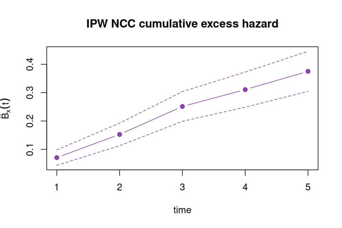

Cumulative excess hazard of the exposure over follow-up estimated from the IPW nested case-control additive-hazards model, with a pointwise 95% confidence band. The curve rises roughly linearly, indicating an approximately constant excess rate.

Each estimator identifies exactly one scale, so asking for another is rejected:

Code

contrast(fit_aft, type = "hr")
#> Error in `contrast()`:
#> ! The IPW NCC accelerated failure time model reports a time ratio, not `type = "hr"`.
#> ℹ Use `type = "af"` (the default for `ipw_aft`).

References

Borgan, Ørnulf, and Bryan Langholz. 1997. “Estimation of Excess Risk from Case-Control Data Using Aalen’s Linear Regression Model.” Biometrics 53 (2): 690–97. https://doi.org/10.2307/2533968.

Kang, Sangwook, Wenbin Lu, and Mengling Liu. 2017. “Efficient Estimation for Accelerated Failure Time Model Under Case-Cohort and Nested Case-Control Sampling.” Biometrics 73 (1): 114–23. https://doi.org/10.1111/biom.12573.

Lin, Danyu Y., and Zhiliang Ying. 1994. “Semiparametric Analysis of the Additive Risk Model.” Biometrika 81 (1): 61–71. https://doi.org/10.1093/biomet/81.1.61.

Saarela, Olli, Sangita Kulathinal, Elja Arjas, and Esa Läärä. 2008. “Nested Case-Control Data Utilized for Multiple Outcomes: A Likelihood Approach and Alternatives.” Statistics in Medicine 27 (28): 5991–6008. https://doi.org/10.1002/sim.3416.

Samuelsen, Sven Ove. 1997. “A Pseudolikelihood Approach to Analysis of Nested Case-Control Studies.” Biometrika 84 (2): 379–94. https://doi.org/10.1093/biomet/84.2.379.

Støer, Nathalie C., and Sven Ove Samuelsen. 2012. “Comparison of Estimators in Nested Case-Control Studies with Multiple Outcomes.” Lifetime Data Analysis 18 (3): 261–83. https://doi.org/10.1007/s10985-012-9214-8.

Støer, Nathalie C., and Sven Ove Samuelsen. 2013. “Inverse Probability Weighting in Nested Case-Control Studies with Additional Matching—a Simulation Study.” Statistics in Medicine 32 (30): 5328–39. https://doi.org/10.1002/sim.6019.