---
title: "Longitudinal survival via ICE hazards with survatr"
code-fold: show
code-tools: true
vignette: >
%\VignetteIndexEntry{Longitudinal survival via ICE hazards with survatr}
%\VignetteEngine{quarto::html}
%\VignetteEncoding{UTF-8}
bibliography: references.bib
---
```{r}
#| include: false
knitr::opts_chunk$set(collapse = TRUE, comment = "#>")
set.seed(2026)
```
Point-treatment g-computation (`estimator = "gcomp"` / `"ipw"`) handles a
**point** treatment fixed at baseline. When the treatment varies over time and
there is **treatment–confounder feedback** — a time-varying covariate that both
responds to past treatment and drives future treatment and the hazard — a
point-treatment hazard model is biased, and no single weighted MSM recovers the
counterfactual curve. survatr's **longitudinal ICE-hazard** engine
(`estimator = "ice"`) solves this with iterated conditional expectations (ICE)
on the discrete-time hazard [@zivich2024ice].
This vignette explains the ICE backward sweep, the longitudinal ICE-hazard
arguments (`confounders_tv`, `history`), and shows the estimator recovering the
longitudinal g-formula truth on a feedback DGP that fools the naive curve.
## Why ICE, not a single hazard model
With feedback, a time-varying confounder $L_k$ is simultaneously a **confounder**
of later treatment and a **mediator** of earlier treatment. Conditioning on it
(as a covariate-adjusted hazard would) blocks the causal path; ignoring it
leaves confounding. The g-formula resolves this by standardizing sequentially.
survatr implements the **iterated conditional expectation** form: rather than
modelling every time-varying covariate (forward simulation, à la `gfoRmula`),
ICE models the outcome only, iterating backward from the horizon. At each step
the pseudo-outcome is the **survival tail** under the intervention,
$$
\tilde{Y}_k = D_k + (1 - D_k)\, q_{k+1},
$$
where $D_k$ is the cumulative event indicator and $q_{k+1}$ the predicted
survival probability from the next step. The final step is a binomial fit on the
observed event; earlier steps are quasibinomial fits on the continuous tail
pseudo-outcome. Inference is a stacked-EE sandwich across the per-step models
(or a per-id bootstrap).
## A treatment–confounder-feedback DGP
We simulate a discrete-time survival process following the Ch. 21 structure of
@hernan_whatif, where the time-varying confounder $L_k$ drives both the current
treatment $A_k$ and the hazard, and past treatment $A_{k-1}$ feeds forward into
$L_k$:
$$
\begin{aligned}
L_k &\sim N(\mu_L L_{k-1} + \mu_A A_{k-1},\; 1) \\
A_k &\sim \text{Bernoulli}\!\bigl(\text{logit}^{-1}(g_L L_k + g_A A_{k-1})\bigr) \\
\text{logit}\, h_k &= \alpha_0 + \beta_L L_k + \beta_A A_k,
\end{aligned}
$$
with $\beta_A < 0$ (treatment is protective). Rows at and after the first event
are padded to keep the person-period grid rectangular.
```{r}
#| message: false
library(causatr) # attach first so survatr's contrast() generic dispatches
library(survatr)
library(data.table)
# Shared parameters (feedback structure).
p <- list(g_L = 0.6, g_A = -0.3, mu_L = 0.4, mu_A = 0.5,
a0 = -2, bL = 0.8, bA = -0.7, a_prev0 = 0)
sim_feedback <- function(n = 3000L, K = 4L, seed = 1L, p = p) {
set.seed(seed)
rbindlist(lapply(seq_len(n), function(i) {
L <- A <- numeric(K)
Y <- integer(K)
l_prev <- 0
a_prev <- p$a_prev0
failed <- NA_integer_
for (k in seq_len(K)) {
L[k] <- rnorm(1, p$mu_L * l_prev + p$mu_A * a_prev, 1)
A[k] <- rbinom(1, 1L, plogis(p$g_L * L[k] + p$g_A * a_prev))
Y[k] <- rbinom(1, 1L, plogis(p$a0 + p$bL * L[k] + p$bA * A[k]))
l_prev <- L[k]
a_prev <- A[k]
if (Y[k] == 1L) { failed <- k; break }
}
if (!is.na(failed) && failed < K) { # pad post-event rows
idx <- (failed + 1L):K
L[idx] <- L[failed]; A[idx] <- A[failed]; Y[idx] <- 0L
}
data.table(id = i, t = seq_len(K), L = L, A = A, Y = Y)
}))
}
dat <- sim_feedback(p = p)
head(dat, 6)
```
## Fitting the longitudinal ICE-hazard model
Pass `estimator = "ice"`. The longitudinal ICE-hazard arguments split the
adjustment set:
- **`confounders`** — *baseline* (time-invariant) covariates, never lagged.
Here there are none, so `~ 1`.
- **`confounders_tv`** — *time-varying* covariates, lag-expanded at each
backward step (e.g. `~ L` builds `L + lag1_L + ...`).
- **`history`** — the Markov lag order. `Inf` (default) uses the full available
history; an integer (e.g. `history = 1`) restricts to a first-order Markov
structure.
The treatment must be **numeric** (binary or a linear dose) and may vary within
id. `surv_fit()` fits no model itself for ICE — the per-step models are fit
lazily inside `contrast()` per (intervention, horizon).
```{r}
fit <- surv_fit(
dat,
outcome = "Y",
treatment = "A",
confounders = ~ 1, # no baseline confounders here
confounders_tv = ~ L, # time-varying confounder, lag-expanded
id = "id",
time = "t",
estimator = "ice"
)
fit
```
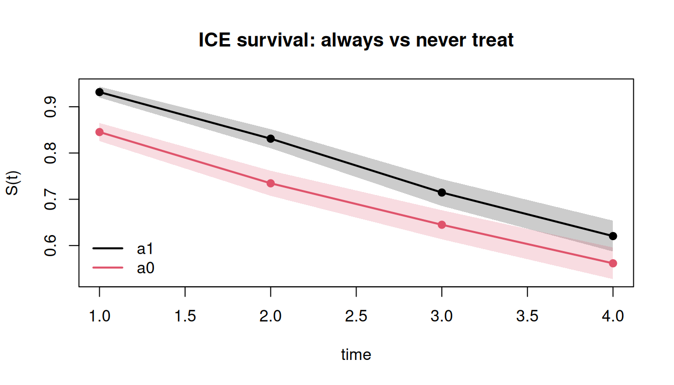
## Counterfactual survival under static strategies
A static strategy "always treat" (`static(1)`) vs "never treat" (`static(0)`)
sets $A_k$ at every period; ICE standardizes over the evolving confounder
history. The protective treatment yields higher survival under `a1`.
```{r}
res_surv <- contrast(
fit,
interventions = list(a1 = static(1), a0 = static(0)),
times = 1:4,
type = "survival",
ci_method = "sandwich"
)
res_surv
```
```{r}
#| fig-width: 7
#| fig-height: 4
#| fig-alt: "longitudinal ICE-hazard ICE counterfactual survival under always-treat versus never-treat."
plot(res_surv, main = "ICE survival: always vs never treat")
```
## ICE corrects feedback bias
The point of the longitudinal ICE-hazard engine is that a **point-treatment**
hazard model is biased under feedback, while ICE is not. A naive point-treatment
g-computation treats $A$ as if it
were fixed at baseline (it warns that the treatment is time-varying) and adjusts
for $L$ as an ordinary confounder — which blocks the mediated causal path. Its
`a1` survival curve diverges from the ICE curve:
```{r}
fit_naive <- suppressWarnings(surv_fit(
dat, "Y", "A", ~ L, "id", "t",
time_formula = ~ factor(t), estimator = "gcomp"
))
s_naive <- contrast(
fit_naive, interventions = list(a1 = static(1)),
times = 1:4, type = "survival"
)$estimates
ice_a1 <- res_surv$estimates[intervention == "a1"][order(time)]
data.table(
time = ice_a1$time,
ice = round(ice_a1$s_hat, 3),
naive_gc = round(s_naive[order(time)]$s_hat, 3)
)[] # `[]` forces auto-print of a function-returned data.table
```
Only the ICE g-formula curve targets $S^{a=1}(t)$ correctly; the naive
point-treatment curve is biased because it conditions on the feedback variable
$L$.
## Risk difference, risk ratio, RMST
All the point-treatment estimand types are available on a longitudinal
ICE-hazard fit. The stacked-EE
sandwich propagates the cross-step influence-function cascade through the
cumulative-product survival curve.
```{r}
for (ty in c("risk_difference", "risk_ratio", "rmst_difference")) {
rr <- contrast(
fit,
interventions = list(a1 = static(1), a0 = static(0)),
times = 4L, type = ty, reference = "a0", ci_method = "sandwich"
)
cat(sprintf("%-16s estimate = %+.4f (se = %.4f)\n",
ty, rr$contrasts$estimate, rr$contrasts$se))
}
```
## Sandwich vs bootstrap
The survival influence-function chain carries a $(1 - D_k)$ failure
carry-forward factor that a terminal-outcome ICE chain omits; reusing the latter
verbatim over-covers at later horizons. The sandwich and the per-id bootstrap
should agree at every horizon:
```{r}
sw <- contrast(
fit, interventions = list(a1 = static(1), a0 = static(0)),
times = 1:4, type = "survival", ci_method = "sandwich"
)$estimates
bo <- contrast(
fit, interventions = list(a1 = static(1), a0 = static(0)),
times = 1:4, type = "survival", ci_method = "bootstrap",
n_boot = 200L, seed = 42L
)$estimates
merge(
sw[, .(intervention, time, se_sandwich = se)],
bo[, .(intervention, time, se_bootstrap = se)],
by = c("intervention", "time")
)[]
```
## Dynamic strategies
ICE also handles genuinely longitudinal **dynamic** strategies — treat as a
function of the evolving covariate. Here, "treat whenever the current confounder
is positive":
```{r}
res_dyn <- contrast(
fit,
interventions = list(
treat_if_L = dynamic(function(data, trt) as.integer(data$L > 0)),
never = static(0)
),
times = 1:4,
type = "risk_difference",
reference = "never",
ci_method = "sandwich"
)
res_dyn$contrasts[]
```
Only the current-period treatment is intervened; the lag columns carry the
**observed** past treatment, as the ICE g-formula requires.
## Scope and rejections
The longitudinal ICE-hazard engine currently supports a numeric treatment with
`static` / `shift` /
`dynamic` strategies and sandwich or bootstrap inference. It rejects, with
classed errors, combinations that need later chunks:
| Trigger | Error class |
|---|---|
| Non-numeric (factor / categorical) treatment | `survatr_ice_treatment_unsupported` |
| `ipsi()` / stochastic intervention | `survatr_ice_intervention_deferred` |
| External / IPCW `weights =` | `survatr_ice_external_weights` |
A baseline-constant treatment is allowed under ICE (it just informs that
point-treatment g-computation is cheaper). Entry (period-1) censoring is handled
by standardizing over the
at-risk-at-baseline population (consistent under MCAR), not by returning an
all-`NA` curve.
## References
::: {#refs}
:::