---
title: "IPW survival with survatr"
code-fold: show
code-tools: true
vignette: >
%\VignetteIndexEntry{IPW survival with survatr}
%\VignetteEngine{quarto::html}
%\VignetteEncoding{UTF-8}
bibliography: references.bib
---
```{r}
#| include: false
knitr::opts_chunk$set(collapse = TRUE, comment = "#>")
set.seed(2026)
```
Inverse-probability weighting (IPW) estimates the counterfactual survival curve
by reweighting the observed data so that confounders are balanced across
treatment groups, then fitting a **weighted marginal hazard MSM**
[@robins2000msmepi] rather than a covariate-adjusted hazard — the IP-weighted
approach to survival analysis of @hernan_whatif, Ch. 17. It is the second of
survatr's two point-treatment estimators
(alongside g-computation) and a methodologically distinct route to the same
estimand — when the two agree you can be more confident in the result.
This vignette covers `estimator = "ipw"` for a **binary point treatment**: the
weight construction, the supported estimands and interventions, sandwich vs
bootstrap inference, and weight truncation.
## How survatr's IPW differs from g-computation
g-computation models the hazard $h(t \mid A, L)$ and standardizes over the
covariate distribution. IPW instead models the **treatment mechanism**
$f(A \mid L)$ and reweights. survatr composes a **stabilized** density-ratio
weight at the baseline (one row per id),
$$
w_i = \frac{f(A_i)}{f(A_i \mid L_i)},
$$
broadcasts the per-id weight onto every person-period row, and fits an
intervention-free weighted marginal hazard MSM
$\text{logit}\, h(t \mid A) = \alpha(t) + \beta_A A$. Because the weighting
removes confounding, the MSM needs only $A$ and the baseline-hazard term
$\alpha(t)$ — no $L$. The treatment model is fit by `propensity_model_fn`
(default `stats::glm`); the hazard MSM by `model_fn`.
## A confounded survival DGP
We simulate person-period data with a constant-ish discrete-time hazard, a
single baseline confounder $L$ that drives **both** treatment assignment and the
hazard, and a genuinely protective treatment ($\beta_A < 0$):
$$
\begin{aligned}
L_i &\sim N(0, 1) \\
A_i \mid L_i &\sim \text{Bernoulli}\!\bigl(\text{logit}^{-1}(\gamma\, L_i)\bigr) \\
\text{logit}\, h_{i,k} &= \alpha_0 + \alpha_k + \beta_A A_i + \beta_L L_i,
\end{aligned}
$$
with first-event truncation and rectangular padding (so every id has one row at
every period). Because $L$ confounds the $A \to Y$ relationship, the unadjusted
survival curve is biased; IPW recovers the counterfactual curve.
```{r}
#| message: false
library(causatr) # attach first so survatr's contrast() generic dispatches
library(survatr)
library(data.table)
sim_confounded <- function(n = 2000L, K = 5L, seed = 1L,
gamma = 0.8, alpha0 = -2, beta_A = -0.6,
beta_L = 0.7) {
set.seed(seed)
L <- rnorm(n)
A <- rbinom(n, 1L, plogis(gamma * L)) # L drives treatment (confounding)
alpha_t <- seq(0, 0.3, length.out = K) # mild per-period baseline drift
rbindlist(lapply(seq_len(n), function(i) {
h <- plogis(alpha0 + alpha_t + beta_A * A[i] + beta_L * L[i])
Y <- rbinom(K, 1L, h)
first <- which(Y == 1L)[1L]
if (!is.na(first) && first < K) Y[(first + 1L):K] <- 0L
data.table(id = i, t = seq_len(K), A = A[i], L = L[i], Y = Y)
}))
}
pp <- sim_confounded()
head(pp, 5)
```
## Fitting the IPW hazard MSM
Pass `estimator = "ipw"`. `confounders` specifies the treatment model
$f(A \mid L)$; the weighted MSM uses only $A$.
```{r}
fit <- surv_fit(
pp,
outcome = "Y",
treatment = "A",
confounders = ~ L,
id = "id",
time = "t",
time_formula = ~ factor(t), # non-parametric baseline hazard
estimator = "ipw"
)
fit
```
### The stabilized weights
`fit$weights` holds the per-person-period broadcast weight. Stabilization
centres the weights near 1, and the weight is constant within an id (the
baseline density ratio is broadcast onto all of that id's rows):
```{r}
w_dt <- data.table(id = pp$id, w = fit$weights)
summary(unique(w_dt)$w)
# the weight is constant within each id (one density ratio, broadcast)
all(w_dt[, uniqueN(w), by = id]$V1 == 1L)
```
## Survival curves
`contrast()` produces the time-indexed counterfactual survival curve under each
intervention. Interventions are constructed with `causatr::static()`.
```{r}
res_surv <- contrast(
fit,
interventions = list(a1 = static(1), a0 = static(0)),
times = 1:5,
type = "survival",
ci_method = "sandwich"
)
res_surv
```
```{r}
#| fig-width: 7
#| fig-height: 4
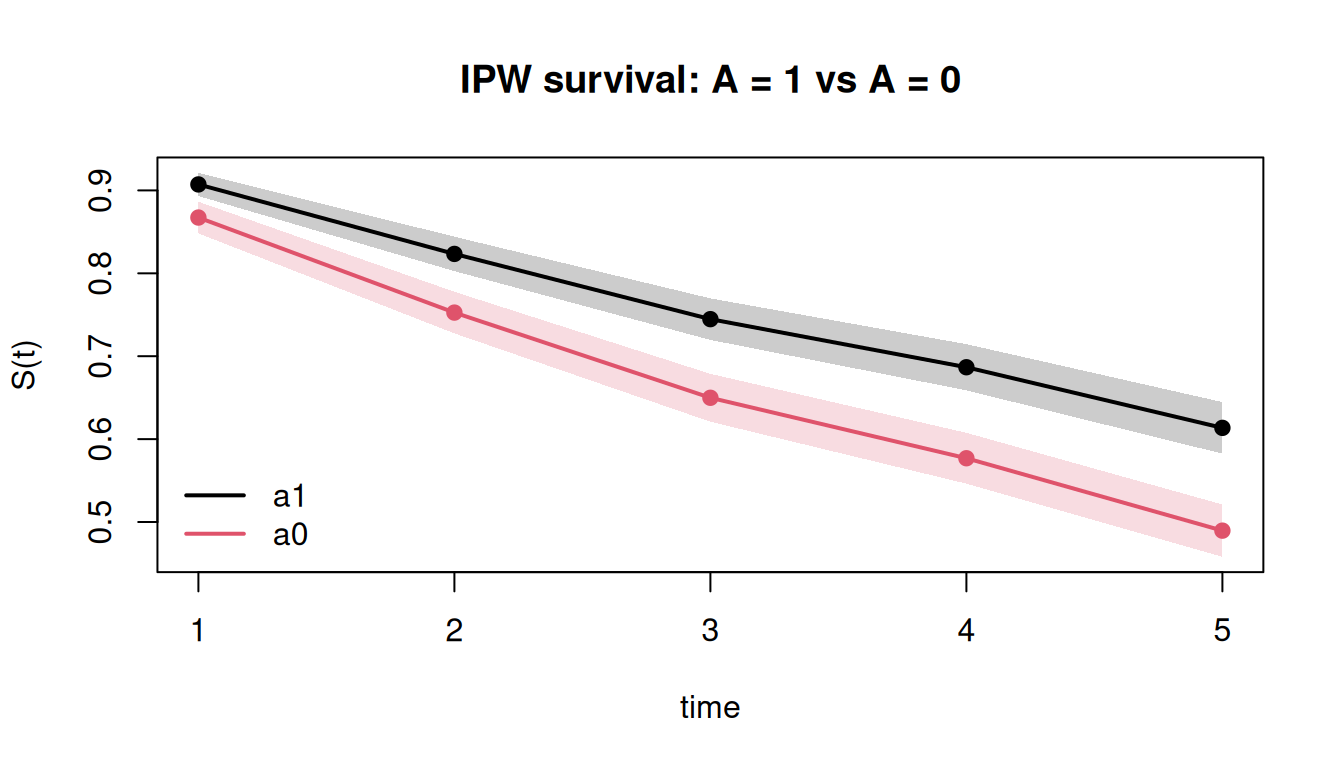
#| fig-alt: "IPW counterfactual survival curves under treatment versus no treatment."
plot(res_surv, main = "IPW survival: A = 1 vs A = 0")
```
Because treatment is protective, survival under `a1` sits above `a0`.
## Risk difference and risk ratio
The pairwise estimands (`risk_difference`, `risk_ratio`, `rmst_difference`) need
a `reference` intervention. The risk-ratio CI is built on the log scale.
```{r}
res_rd <- contrast(
fit,
interventions = list(a1 = static(1), a0 = static(0)),
times = 1:5,
type = "risk_difference",
reference = "a0",
ci_method = "sandwich"
)
res_rd$contrasts[] # `[]` forces auto-print of a function-returned data.table
```
```{r}
res_rr <- contrast(
fit,
interventions = list(a1 = static(1), a0 = static(0)),
times = 1:5,
type = "risk_ratio",
reference = "a0",
ci_method = "sandwich"
)
res_rr$contrasts[]
```
## Sandwich vs bootstrap inference
The IPW sandwich is a **two-stage stacked estimating-equation** variance: it
accounts for estimation of the treatment model by subtracting a treatment-model
correction from the naive weights-as-known sandwich. For stabilized weights this
makes the SE *narrower* than treating the weights as fixed. The nonparametric
bootstrap resamples ids (all of an id's rows together) and refits both the
treatment model and the hazard MSM per replicate; the two agree closely.
```{r}
res_boot <- contrast(
fit,
interventions = list(a1 = static(1), a0 = static(0)),
times = 1:5,
type = "risk_difference",
reference = "a0",
ci_method = "bootstrap",
n_boot = 200L,
seed = 42L
)
# Sandwich vs bootstrap SE at each period.
data.table(
time = res_rd$contrasts$time,
se_sand = res_rd$contrasts$se,
se_boot = res_boot$contrasts$se
)[]
```
## Dynamic interventions
Beyond `static()`, IPW supports `dynamic()` rules: each id is assigned a
treatment value as a function of its baseline covariates. The rule receives the
data and the treatment vector and returns the assigned treatment.
```{r}
res_dyn <- contrast(
fit,
interventions = list(
treat_high = dynamic(function(data, trt) as.integer(data$L > 0)),
none = static(0)
),
times = 1:5,
type = "risk_difference",
reference = "none",
ci_method = "sandwich"
)
res_dyn$contrasts[]
```
## Weight truncation
When the propensity model yields extreme density ratios (near-positivity
violations, strong confounding), the IPW estimator can be unstable. The `trim`
argument on `surv_fit()` winsorizes the per-id stabilized weights at a quantile
[@cole2008constructing] **before** they are broadcast onto the person-period rows;
the resolved cutoff is held fixed and reused by the sandwich variance.
```{r}
fit_trim <- surv_fit(
pp, "Y", "A", ~ L, "id", "t",
time_formula = ~ factor(t), estimator = "ipw",
trim = 0.99 # winsorize at the 99th percentile of the weights
)
c(max_raw = max(fit$weights), max_trim = max(fit_trim$weights),
cutoff = fit_trim$trim_threshold)
```
`trim = NULL` (the default) applies no truncation; an untrimmed fit records
`trim_threshold = NA`.
## What IPW rejects
survatr's IPW path is deliberately narrow for now and rejects unsupported
combinations with **classed** errors rather than fitting something misleading:
| Trigger | Error class |
|---|---|
| Continuous treatment | `survatr_ipw_treatment_unsupported` |
| Treatment varying within id | `survatr_ipw_time_varying_treatment` |
| Constant treatment (no variation → undefined weights) | `survatr_ipw_no_treatment_variation` |
| `ipsi()` intervention | `survatr_ipw_ipsi_deferred` |
| External `weights =` composed with IPW (transport) | `survatr_ipw_external_weights` |
For a time-varying treatment, use `estimator = "ice"` — see `vignette("ice")`.
## References
::: {#refs}
:::