Introduction to survatr

survatr extends the causatr engine to time-to-event outcomes via three building blocks:

Pooled-logistic hazard g-computation on person-period data: $\text{logit}\, h(t \mid A, L) = \alpha(t) + \beta_A A + \beta_L L$, with survival cumulated across periods as $\hat{S}^a_i(t) = \prod_{k \leq t}(1 - \hat{h}^a_{i,k})$.
Delta-method sandwich variance that propagates per-row influence functions through the cumulative product into a cross-time covariance matrix on the survival curve.
Individual-level nonparametric bootstrap that resamples ids (all of each id’s person-period rows together) and refits the hazard model per replicate.

The estimand is a curve (survival, risk, RMST) or a contrast of curves (risk difference, risk ratio, RMST difference), not a scalar. The entire API returns time-indexed data.tables.

Two-step API

All analyses follow the same two-step pattern that causatr users will recognise:

# Step 1: Fit the hazard model once
fit <- surv_fit(
  data,
  outcome     = "Y",
  treatment   = "A",
  confounders = ~ L1 + L2,
  id          = "id",
  time        = "t",
  censoring   = "C",
  time_formula = ~ splines::ns(t, 4)  # alpha(t) baseline hazard
)

# Step 2: Contrast many interventions cheaply on the same fit
result <- contrast(
  fit,
  interventions = list(
    treated = causatr::static(1),
    control = causatr::static(0)
  ),
  times       = seq(0, 120, by = 12),
  type        = "risk_difference",
  reference   = "control",
  ci_method   = "sandwich"
)

Quick example

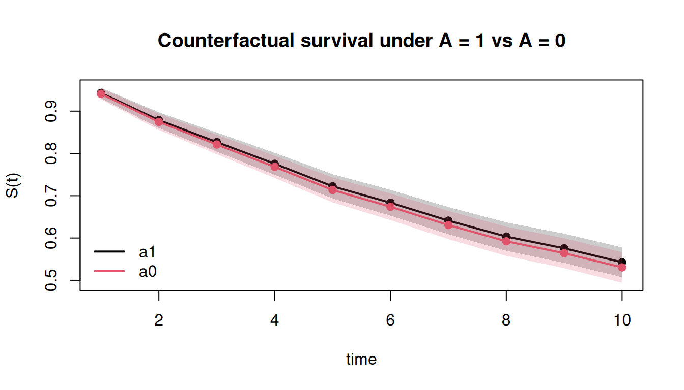
The example below uses a simulated DGP: a constant discrete-time hazard of 6% per period, a single binary treatment with no causal effect, and one normal-distributed confounder that jointly affects the propensity of treatment and the hazard rate. Under this DGP the counterfactual survival under either intervention converges to $(1 - 0.06)^t$, so we can check the point estimates against the closed form.

Code

## Attach `causatr` first so survatr's `contrast()` generic shadows
## causatr's scalar-outcome `contrast()` and dispatches correctly on
## `survatr_fit` objects. Call `causatr::contrast()` explicitly if you
## need the causatr path while survatr is loaded.
library(causatr)
library(survatr)
library(data.table)

## Simulate person-period data with a constant hazard and a confounder L.
sim_pp <- function(n = 1500L, K = 10L, h = 0.06, seed = 1L) {
  set.seed(seed)
  L <- rnorm(n)                                 # single baseline confounder
  A <- rbinom(n, 1L, plogis(0.3 * L))           # L affects treatment
  rows <- vector("list", n)
  for (i in seq_len(n)) {
    Y <- rbinom(K, 1L, h)                        # hazard independent of A (null)
    first <- which(Y == 1L)[1L]
    if (!is.na(first) && first < K) Y[(first + 1L):K] <- 0L
    rows[[i]] <- data.table::data.table(
      id = i, t = seq_len(K), A = A[i], L = L[i], Y = Y
    )
  }
  data.table::rbindlist(rows)
}

pp <- sim_pp()
head(pp, 5)
#>       id     t     A          L     Y
#>    <int> <int> <int>      <num> <int>
#> 1:     1     1     1 -0.6264538     0
#> 2:     1     2     1 -0.6264538     0
#> 3:     1     3     1 -0.6264538     0
#> 4:     1     4     1 -0.6264538     0
#> 5:     1     5     1 -0.6264538     0

Fit the hazard model

Code

fit <- surv_fit(
  pp,
  outcome      = "Y",
  treatment    = "A",
  confounders  = ~ L,
  id           = "id",
  time         = "t",
  time_formula = ~ factor(t)   # non-parametric baseline hazard
)
fit
#> <survatr_fit>
#>   Track:       A
#>   Estimator:   gcomp
#>   Family:      binomial
#>   Outcome:     Y
#>   Treatment:   A
#>   ID:          id
#>   Time:        t
#>   Censoring:   none
#>   N:           1500 individuals, 15000 PP rows (11423 at risk)
#>   Time grid:   [1, 10] (10 unique times)

Survival curves under two interventions

Code

res_surv <- contrast(
  fit,
  interventions = list(
    a1 = causatr::static(1),
    a0 = causatr::static(0)
  ),
  times     = 1:10,
  type      = "survival",
  ci_method = "sandwich"
)
res_surv
#> <survatr_result>
#>   Type:        survival
#>   Reference:   (none)
#>   CI method:   sandwich
#>   Time grid:   [1, 10] (10 unique times)
#>   Estimates:   20 rows
#>   Contrasts:   0 rows
#> 
#>     intervention  time     s_hat   risk_hat          se  ci_lower  ci_upper
#>           <char> <int>     <num>      <num>       <num>     <num>     <num>
#>  1:           a1     1 0.9429846 0.05701541 0.006267503 0.9307005 0.9552687
#>  2:           a1     2 0.8786721 0.12132791 0.009437176 0.8601756 0.8971686
#>  3:           a1     3 0.8267793 0.17322073 0.011515336 0.8042096 0.8493489
#>  4:           a1     4 0.7754882 0.22451176 0.013224880 0.7495680 0.8014085
#>  5:           a1     5 0.7221593 0.27784075 0.014669052 0.6934084 0.7509101
#>  6:           a1     6 0.6832754 0.31672462 0.015549770 0.6527984 0.7137524
#>  7:           a1     7 0.6410406 0.35895942 0.016384880 0.6089268 0.6731544
#>  8:           a1     8 0.6033769 0.39662309 0.017148193 0.5697671 0.6369867
#>  9:           a1     9 0.5756057 0.42439434 0.017615190 0.5410805 0.6101308
#> 10:           a1    10 0.5425151 0.45748489 0.018002313 0.5072312 0.5777990
#>         n
#>     <int>
#>  1:  1500
#>  2:  1500
#>  3:  1500
#>  4:  1500
#>  5:  1500
#>  6:  1500
#>  7:  1500
#>  8:  1500
#>  9:  1500
#> 10:  1500

Code

plot(res_surv, main = "Counterfactual survival under A = 1 vs A = 0")

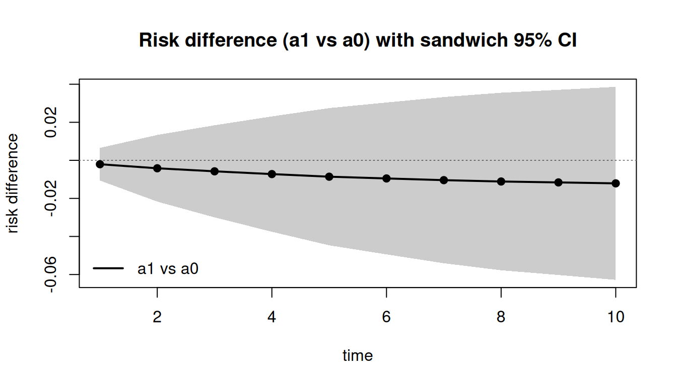
Risk difference with sandwich CI

Code

res_rd <- contrast(
  fit,
  interventions = list(
    a1 = causatr::static(1),
    a0 = causatr::static(0)
  ),
  times     = 1:10,
  type      = "risk_difference",
  reference = "a0",
  ci_method = "sandwich"
)
res_rd$contrasts[] # `[]` forces auto-print of a function-returned data.table
#>     contrast  time     estimate          se    ci_lower    ci_upper
#>       <char> <int>        <num>       <num>       <num>       <num>
#>  1: a1 vs a0     1 -0.002041379 0.004378228 -0.01062255 0.006539789
#>  2: a1 vs a0     2 -0.004171571 0.008932308 -0.02167857 0.013335430
#>  3: a1 vs a0     3 -0.005770166 0.012348210 -0.02997221 0.018431881
#>  4: a1 vs a0     4 -0.007225694 0.015461865 -0.03753039 0.023079005
#>  5: a1 vs a0     5 -0.008595905 0.018396179 -0.04465175 0.027459943
#>  6: a1 vs a0     6 -0.009513415 0.020361869 -0.04942194 0.030395114
#>  7: a1 vs a0     7 -0.010408541 0.022278540 -0.05407368 0.033256595
#>  8: a1 vs a0     8 -0.011120983 0.023800384 -0.05776888 0.035526913
#>  9: a1 vs a0     9 -0.011596826 0.024817563 -0.06023836 0.037044704
#> 10: a1 vs a0    10 -0.012090341 0.025873948 -0.06280235 0.038621665

Code

plot(res_rd, main = "Risk difference (a1 vs a0) with sandwich 95% CI")

The DGP has no treatment effect, so the risk-difference CI should comfortably cover 0 at every time point.

Estimand menu

Pass any of the following to type =:

`type`	Estimand	Shape of result
`"survival"`	$\hat{S}^a(t)$	One row per (intervention, time)
`"risk"`	$1 - \hat{S}^a(t)$	One row per (intervention, time)
`"rmst"`	$\int_0^t \hat{S}^a(u)\,du$	One row per (intervention, time)
`"risk_difference"`	$\hat{R}^{a_1}(t) - \hat{R}^{a_0}(t)$	Pairwise contrasts
`"risk_ratio"`	$\hat{R}^{a_1}(t) / \hat{R}^{a_0}(t)$	Pairwise contrasts (log-scale CI)
`"rmst_difference"`	$\mathrm{RMST}^{a_1}(t) - \mathrm{RMST}^{a_0}(t)$	Pairwise contrasts

"survival", "risk", and "rmst" return an empty contrasts table (stable schema); the three pairwise types fill it.

Intervention types

Interventions are constructed via causatr:

Constructor	Description	Example
`causatr::static(value)`	Set treatment to a fixed value	`static(1)`
`causatr::shift(delta)`	Add a constant to observed treatment	`shift(0.5)`
`causatr::scale_by(factor)`	Multiply observed treatment	`scale_by(0.5)`
`causatr::threshold(lower, upper)`	Clamp treatment within bounds	`threshold(0, 20)`
`causatr::dynamic(rule)`	Apply a user-defined rule	`dynamic(\(d, a) ifelse(d$L > 0, 1, 0))`

The dynamic() rule and IPW (estimator = "ipw") are demonstrated in vignette("ipw"); longitudinal time-varying treatments via Track B ICE (estimator = "ice") are covered in vignette("ice"). IPW-style stochastic (ipsi()) interventions ship in a later chunk.

Inference methods

`ci_method`	Description
`"none"`	Point estimates only (default). `se` / `ci_*` columns are `NA_real_`.
`"sandwich"`	Delta-method cross-time influence function aggregation through the cumulative product. Pointwise Wald bands. Fast (single pass).
`"bootstrap"`	Nonparametric bootstrap with per-id resampling. Percentile (default) or Wald CIs. Slower; required for non-GLM outcome fitters (e.g. `mgcv::gam`).

Code

res_boot <- contrast(
  fit,
  interventions = list(
    a1 = causatr::static(1),
    a0 = causatr::static(0)
  ),
  times     = 1:10,
  type      = "risk_difference",
  reference = "a0",
  ci_method = "bootstrap",
  n_boot    = 200L,
  seed      = 42L
)
head(res_boot$contrasts, 3)
#> Key: <contrast, time>
#>    contrast  time     estimate          se    ci_lower    ci_upper
#>      <char> <int>        <num>       <num>       <num>       <num>
#> 1: a1 vs a0     1 -0.002041379 0.004091117 -0.01035280 0.006202343
#> 2: a1 vs a0     2 -0.004171571 0.008360997 -0.02275464 0.012317831
#> 3: a1 vs a0     3 -0.005770166 0.011535107 -0.03143288 0.016800506

Sandwich and bootstrap SEs match each other — and the true sampling SD — to within 1–2% on this DGP at n = 1500 (confirmed via a 300-replicate empirical-SD oracle; see tests/testthat/test-bootstrap-survival.R).

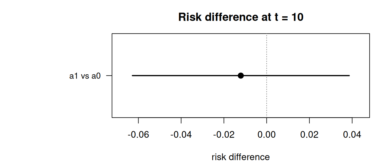
Extracting results

tidy(), plot(), print(), and forrest() all dispatch on the time-indexed survatr_result shape:

Code

res_td <- tidy(res_rd)
head(res_td, 6)
#>   intervention contrast time estimand   estimate          se   ci_lower
#> 1           a1     <NA>    1 risk_hat 0.05701541 0.006267503 0.04473133
#> 2           a1     <NA>    2 risk_hat 0.12132791 0.009437176 0.10283139
#> 3           a1     <NA>    3 risk_hat 0.17322073 0.011515336 0.15065108
#> 4           a1     <NA>    4 risk_hat 0.22451176 0.013224880 0.19859147
#> 5           a1     <NA>    5 risk_hat 0.27784075 0.014669052 0.24908993
#> 6           a1     <NA>    6 risk_hat 0.31672462 0.015549770 0.28624763
#>     ci_upper
#> 1 0.06929949
#> 2 0.13982444
#> 3 0.19579037
#> 4 0.25043205
#> 5 0.30659156
#> 6 0.34720161

Code

forrest(res_rd, t_ref = 10, main = "Risk difference at t = 10")

Reserved columns and error surface

survatr reserves column names prefixed with .survatr_* for internal bookkeeping (.survatr_prev_event, .survatr_prev_cens). User-data collisions produce survatr_reserved_col.

All rejection paths raise classed errors with the survatr_* prefix so downstream code can pattern-match on class rather than English:

Class	Trigger
`survatr_bad_interventions`	Empty / unnamed / duplicate-named / wrong-type `interventions`, or a pairwise-contrast `type` with a single intervention
`survatr_bad_times`	Non-numeric / empty / NA `times`
`survatr_time_extrapolation`	`times` outside `fit$time_grid`
`survatr_bad_reference`	`reference` not in `interventions` names
`survatr_bad_ci_method`	`ci_method` not in `{"none", "sandwich", "bootstrap"}`
`survatr_bad_conf_level`	`conf_level` outside `(0, 1)`
`survatr_bad_n_boot` / `survatr_bad_boot_ci` / `survatr_bad_parallel`	Bootstrap argument misuse
`survatr_matching_rejected`	`estimator = "matching"` (use `survival::coxph(..., weights, cluster)` instead)
`survatr_bad_na_action`	`na.action = na.exclude` (silently corrupts sandwich variance)
`survatr_competing_misuse`	Non-`NULL` `competing` argument (cause-specific path ships later)

Learning more

This vignette covered Track A g-computation. Two further estimators are implemented and have dedicated vignettes:

Track A under IPW (vignette("ipw")) — stabilized density-ratio weights broadcast onto person-period rows, fitting a weighted marginal hazard MSM.
Track B (ICE hazards) (vignette("ice")) — longitudinal survival for a time-varying treatment via iterated conditional expectations (Zivich et al. 2024), with the hazard indicator at the final period and a survival-tail pseudo-outcome at earlier periods.

survatr’s full scope is laid out in SURVIVAL_PACKAGE_HANDOFF.md. Upcoming chunks will add:

Competing risks — parallel cause-specific hazards + cumulative incidence decomposition.
NHEFS Chapter 17 replication — the Hernán & Robins running example with the 120-month survival curves and the ≈ 0.2% risk difference target.

References

Hernán MA, Robins JM (2025). Causal Inference: What If. Chapman & Hall/CRC. Chapter 17 (survival analysis via IP weighting and standardisation).
Zivich PN, Ross RK, Shook-Sa BE, Cole SR, Edwards JK (2024). Empirical sandwich variance estimator for iterated conditional expectation g-computation. Statistics in Medicine 43:5562–5572.
D’Agostino RB, Lee ML, Belanger AJ, Cupples LA, Anderson K, Kannel WB (1990). Relation of pooled logistic regression to time-dependent Cox regression analysis: the Framingham Heart Study. Statistics in Medicine 9:1501–1515.