---
title: "G-computation with causatr"
code-fold: show
code-tools: true
vignette: >
%\VignetteIndexEntry{G-computation with causatr}
%\VignetteEngine{quarto::html}
%\VignetteEncoding{UTF-8}
bibliography: references.bib
nocite: |
@diaz2012population
---
```{r}
#| include: false
knitr::opts_chunk$set(collapse = TRUE, comment = "#>")
```
G-computation (the parametric g-formula) estimates causal effects by fitting a
model for the outcome conditional on treatment and confounders, then
standardising predictions over the target population under each hypothetical
intervention. This vignette demonstrates g-computation in causatr using the
NHEFS dataset from @hernan_whatif, covering every supported combination
of treatment type, outcome type, contrast scale, and inference method for
time-fixed treatments.
## Data: NHEFS
The examples in this vignette use the **NHEFS** (National Health and
Nutrition Examination Survey — Epidemiologic Follow-up Study) dataset,
the running example in @hernan_whatif. The assumed causal
structure is:
- **Treatment ($A$):** `qsmk` — quit smoking between 1971 and 1982 (binary: 0/1).
- **Outcome ($Y$):** `wt82_71` — weight change in kg over the same period
(continuous). A derived binary version, `gained_weight` ($\mathbf{1}\{Y > 0\}$),
is used in the binary outcome sections.
- **Confounders ($L$):** sex, age, race, education, smoking intensity
(cigarettes/day), years smoked, exercise, physical activity, and baseline
weight. These jointly affect both the probability of quitting and the
subsequent weight change.
- **Censoring:** the `censored` column flags individuals lost to follow-up.
Censored rows are excluded from model fitting; predictions are
standardised over the full target population.
Structural causal model (assumed):
$$
\begin{aligned}
L &\sim F_L \\
A &\sim \text{Bernoulli}\!\bigl(\text{logit}^{-1}(\alpha_0 + \alpha_L^\top L)\bigr) \\
Y &= \beta_0 + \beta_A A + \beta_L^\top L + \beta_{AL}^\top (A \cdot L) + \varepsilon,
\quad \varepsilon \sim N(0, \sigma^2)
\end{aligned}
$$
The confounders $L$ are common causes of $A$ and $Y$; adjusting for $L$
blocks all backdoor paths, identifying $\mathbb{E}[Y^a]$ via the g-formula.
```{r}
#| message: false
library(causatr)
library(tinytable)
library(tinyplot)

data("nhefs")

nhefs_complete <- nhefs[!is.na(nhefs$wt82_71), ]

nhefs_complete$gained_weight <- as.integer(nhefs_complete$wt82_71 > 0)

nhefs$sex <- factor(nhefs$sex, levels = 0:1, labels = c("Male", "Female"))
nhefs_complete$sex <- factor(
  nhefs_complete$sex,
  levels = 0:1,
  labels = c("Male", "Female")
)
```
We create a binary outcome `gained_weight` (1 if weight increased, 0 otherwise)
for the binary outcome examples below.
## Binary treatment, continuous outcome
This is the core example from @hernan_whatif, Ch. 13: the average
causal effect of quitting smoking (`qsmk`) on weight change (`wt82_71`).
By default, `confounders` specifies the same covariate set for all
model components. Use `confounders_outcome` to specify a different set
for the outcome model when needed (e.g. for AIPW double robustness).
### ATE with sandwich SE
```{r}
fit_gc <- causat(
nhefs,
outcome = "wt82_71",
treatment = "qsmk",
confounders = ~ sex + age + I(age^2) + race + factor(education) +
smokeintensity + I(smokeintensity^2) + smokeyrs + I(smokeyrs^2) +
factor(exercise) + factor(active) + wt71 + I(wt71^2) +
qsmk:smokeintensity,
censoring = "censored",
model_fn = stats::glm
)
res_ate_sw <- contrast(
fit_gc,
interventions = list(quit = static(1), continue = static(0)),
reference = "continue",
type = "difference",
ci_method = "sandwich"
)
res_ate_sw
```
The book reports ATE $\approx$ 3.5 kg (95% CI: 2.6, 4.5).
### ATE with bootstrap SE
```{r}
res_ate_bs <- contrast(
fit_gc,
interventions = list(quit = static(1), continue = static(0)),
reference = "continue",
type = "difference",
ci_method = "bootstrap",
n_boot = 50L
)
res_ate_bs
```
Sandwich and bootstrap SEs should be in close agreement for correctly specified
GLMs.
### ATT estimand
The average treatment effect on the treated (ATT) averages only over individuals
who actually quit smoking. With g-computation, the estimand can be changed in
`contrast()` without refitting.
```{r}
res_att <- contrast(
fit_gc,
interventions = list(quit = static(1), continue = static(0)),
reference = "continue",
estimand = "ATT",
ci_method = "sandwich"
)
res_att
```
### ATC estimand
The average treatment effect on the controls (ATC) averages over those who
continued smoking.
```{r}
res_atc <- contrast(
fit_gc,
interventions = list(quit = static(1), continue = static(0)),
reference = "continue",
estimand = "ATC",
ci_method = "sandwich"
)
res_atc
```
### Subset estimand
A custom subgroup: effect among individuals aged 50 or older.
```{r}
res_sub <- contrast(
fit_gc,
interventions = list(quit = static(1), continue = static(0)),
reference = "continue",
subset = quote(age >= 50),
ci_method = "sandwich"
)
res_sub
```
### Extracting results programmatically
```{r}
coef(res_ate_sw)
confint(res_ate_sw)
```
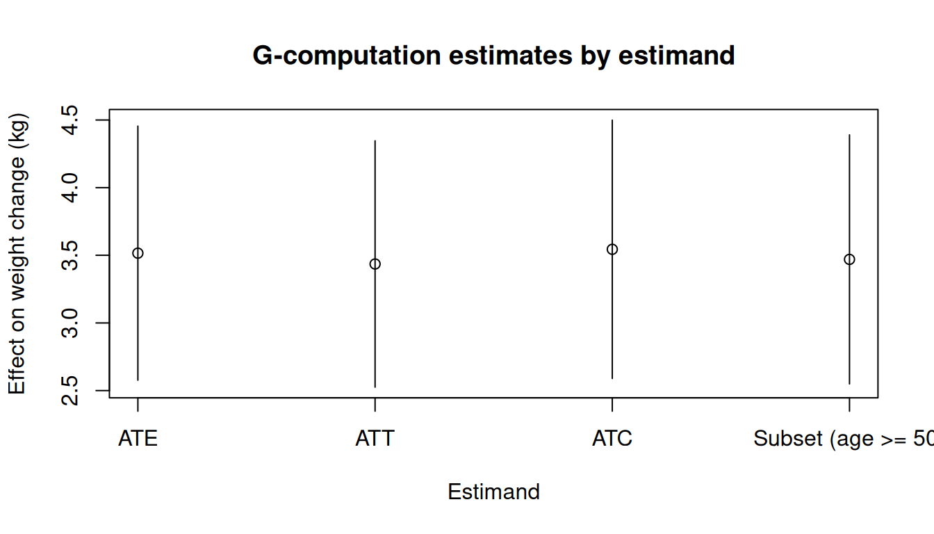
## Comparing estimands
```{r}
#| fig-width: 7
#| fig-height: 4
#| fig-alt: "Point estimates and confidence intervals for ATE, ATT, ATC, and subset estimands from g-computation."
est_df <- data.frame(
  estimand = c("ATE", "ATT", "ATC", "Subset (age >= 50)"),
  estimate = c(
    res_ate_sw$contrasts$estimate[1],
    res_att$contrasts$estimate[1],
    res_atc$contrasts$estimate[1],
    res_sub$contrasts$estimate[1]
  ),
  ci_lower = c(
    res_ate_sw$contrasts$ci_lower[1],
    res_att$contrasts$ci_lower[1],
    res_atc$contrasts$ci_lower[1],
    res_sub$contrasts$ci_lower[1]
  ),
  ci_upper = c(
    res_ate_sw$contrasts$ci_upper[1],
    res_att$contrasts$ci_upper[1],
    res_atc$contrasts$ci_upper[1],
    res_sub$contrasts$ci_upper[1]
  )
)

tinyplot(
  estimate ~ estimand,
  data = est_df,
  type = "pointrange",
  ymin = est_df$ci_lower,
  ymax = est_df$ci_upper,
  xlab = "Estimand",
  ylab = "Effect on weight change (kg)",
  main = "G-computation estimates by estimand"
)
abline(h = 0, lty = 2, col = "grey40")
```
## Binary treatment, binary outcome
Using the `gained_weight` indicator as a binary outcome, we estimate the risk
difference, risk ratio, and odds ratio of quitting smoking on gaining weight.
### Risk difference (sandwich)
```{r}
fit_bin <- causat(
nhefs_complete,
outcome = "gained_weight",
treatment = "qsmk",
confounders = ~ sex + age + I(age^2) + race + factor(education) +
smokeintensity + I(smokeintensity^2) + smokeyrs + I(smokeyrs^2) +
factor(exercise) + factor(active) + wt71 + I(wt71^2) +
qsmk:smokeintensity,
family = "binomial",
model_fn = stats::glm
)
res_rd <- contrast(
fit_bin,
interventions = list(quit = static(1), continue = static(0)),
reference = "continue",
type = "difference",
ci_method = "sandwich"
)
res_rd
```
### Risk difference (bootstrap)
```{r}
res_rd_bs <- contrast(
fit_bin,
interventions = list(quit = static(1), continue = static(0)),
reference = "continue",
type = "difference",
ci_method = "bootstrap",
n_boot = 50L
)
res_rd_bs
```
### Risk ratio
```{r}
res_rr <- contrast(
fit_bin,
interventions = list(quit = static(1), continue = static(0)),
reference = "continue",
type = "ratio",
ci_method = "sandwich"
)
res_rr
```
### Odds ratio
```{r}
res_or <- contrast(
fit_bin,
interventions = list(quit = static(1), continue = static(0)),
reference = "continue",
type = "or",
ci_method = "sandwich"
)
res_or
```
## Continuous treatment
G-computation supports continuous treatments with all intervention types:
`static()` (set to a fixed value), `shift()`, `scale_by()`, `threshold()`,
`dynamic()`, and `NULL` (natural course). Here we use `smokeintensity`
(cigarettes per day) as the treatment and `wt82_71` as the outcome.
```{r}
fit_cont <- causat(
  nhefs,
  outcome = "wt82_71",
  treatment = "smokeintensity",
  confounders = ~ sex + age + I(age^2) + race + factor(education) +
    smokeyrs + I(smokeyrs^2) + factor(exercise) + factor(active) +
    wt71 + I(wt71^2),
  censoring = "censored",
  model_fn = stats::glm
)
```
### Static intervention
Set smoking intensity to fixed values and compare. This answers the question:
what would happen if everyone smoked 5 vs 40 cigarettes per day?
```{r}
res_static <- contrast(
fit_cont,
interventions = list(light = static(5), heavy = static(40)),
reference = "light",
type = "difference",
ci_method = "sandwich"
)
res_static
```
### Shift intervention
Reduce smoking intensity by 10 cigarettes per day for everyone.
```{r}
res_shift <- contrast(
fit_cont,
interventions = list(reduce10 = shift(-10), observed = NULL),
reference = "observed",
type = "difference",
ci_method = "sandwich"
)
res_shift
```
### Scale intervention
Halve each individual's smoking intensity.
```{r}
res_scale <- contrast(
fit_cont,
interventions = list(halved = scale_by(0.5), observed = NULL),
reference = "observed",
type = "difference",
ci_method = "sandwich"
)
res_scale
```
### Threshold intervention
Cap smoking intensity at 20 cigarettes per day for everyone.
```{r}
res_thresh <- contrast(
fit_cont,
interventions = list(cap20 = threshold(0, 20), observed = NULL),
reference = "observed",
type = "difference",
ci_method = "sandwich"
)
res_thresh
```
### Comparing multiple interventions
```{r}
res_multi <- contrast(
fit_cont,
interventions = list(
light = static(5),
reduce10 = shift(-10),
halved = scale_by(0.5),
cap20 = threshold(0, 20),
observed = NULL
),
reference = "observed",
type = "difference",
ci_method = "sandwich"
)
res_multi
```
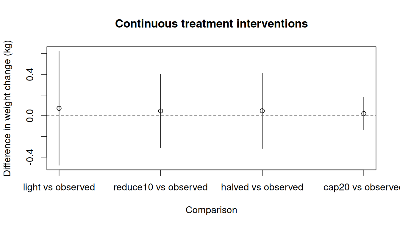
### Visualising intervention effects
```{r}
#| fig-width: 7
#| fig-height: 4
#| fig-alt: "Point estimates and confidence intervals for mean weight change under different smoking intensity interventions."
est <- res_multi$contrasts
tinyplot(
  estimate ~ comparison,
  data = est,
  type = "pointrange",
  ymin = est$ci_lower,
  ymax = est$ci_upper,
  xlab = "Comparison",
  ylab = "Difference in weight change (kg)",
  main = "Continuous treatment interventions"
)
abline(h = 0, lty = 2, col = "grey40")
```
### Dynamic intervention on continuous treatment
A dynamic rule that depends on individual characteristics. Here, heavy smokers
(> 20 cigarettes/day) are reduced to 20, while others keep their observed level.
```{r}
res_dyn_cont <- contrast(
fit_cont,
interventions = list(
capped = dynamic(\(data, trt) pmin(trt, 20)),
observed = NULL
),
reference = "observed",
type = "difference",
ci_method = "sandwich"
)
res_dyn_cont
```
### Continuous treatment with bootstrap
```{r}
res_shift_bs <- contrast(
fit_cont,
interventions = list(reduce10 = shift(-10), observed = NULL),
reference = "observed",
type = "difference",
ci_method = "bootstrap",
n_boot = 50L
)
res_shift_bs
```
## Dynamic intervention
A dynamic intervention assigns treatment based on individual characteristics.
Here, we assign quitting smoking only to individuals who smoked more than 20
cigarettes per day at baseline.
```{r}
res_dyn <- contrast(
fit_gc,
interventions = list(
rule = dynamic(\(data, trt) ifelse(data$smokeintensity > 20, 1, 0)),
all_quit = static(1)
),
reference = "all_quit",
type = "difference",
ci_method = "sandwich"
)
res_dyn
```
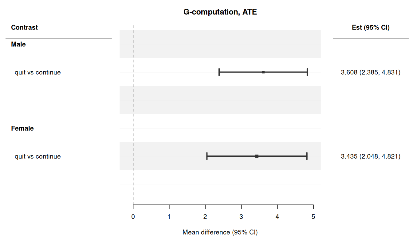
## Effect modification with `by`
The `by` argument stratifies causal effect estimates by levels of a
variable. It averages the fitted model's counterfactual predictions over
each subset — so it only produces *genuine* effect-modification estimates
when the outcome model itself contains an interaction between treatment
and the modifier. Here we refit the model with a `qsmk:sex` term and then
examine how the effect of quitting smoking differs by sex.
```{r}
fit_gc_hte <- causat(
nhefs,
outcome = "wt82_71",
treatment = "qsmk",
confounders = ~ sex + age + I(age^2) + race + factor(education) +
smokeintensity + I(smokeintensity^2) + smokeyrs + I(smokeyrs^2) +
factor(exercise) + factor(active) + wt71 + I(wt71^2) +
qsmk:smokeintensity + qsmk:sex,
censoring = "censored",
model_fn = stats::glm
)
res_by_sex <- contrast(
fit_gc_hte,
interventions = list(quit = static(1), continue = static(0)),
reference = "continue",
type = "difference",
ci_method = "sandwich",
by = "sex"
)
res_by_sex
```
::: {.callout-note}
Without the `qsmk:sex` term in the outcome model, `by = "sex"` would still
run but would return near-identical estimates for both strata (any
remaining variation coming only from indirect interactions like
`qsmk:smokeintensity` combined with differing covariate distributions).
All four estimation methods support `A:modifier` terms: g-comp feeds them
to the outcome model directly, IPW expands the MSM to `Y ~ 1 + modifier`,
matching expands to `Y ~ A + modifier + A:modifier`, and ICE auto-expands
the interaction across treatment lags (`lag1_A:modifier`, etc.).
:::
## Tidy and glance
causatr results work with the broom ecosystem via `tidy()` and `glance()`:
```{r}
tidy(res_ate_sw)
glance(res_ate_sw)
```
## Forest plot
The `plot()` method produces a forest plot using the `forrest` package. Forest
plots are most useful when displaying multiple estimates, such as effect
modification results:
```{r}
#| fig-width: 7
#| fig-height: 4
#| fig-alt: "Forest plot of the effect of quitting smoking on weight change, stratified by sex."
#| eval: !expr requireNamespace("forrest", quietly = TRUE)
plot(res_by_sex)
```
## Categorical treatment (k > 2 levels)
G-computation handles categorical treatments natively by fitting a single
outcome model with the treatment as a factor covariate. `contrast()` then
standardises predictions under each named `static()` level and pairwise
differences are read off against the reference category.
**DGM.** A three-arm trial with one confounder. The treatment is assigned
with fixed probabilities (no confounding of treatment assignment in this
simple example; $L$ is a pure precision variable).
$$
\begin{aligned}
L &\sim N(0,1) \\
A &\sim \text{Categorical}(0.40,\; 0.35,\; 0.25) \quad\text{levels } \{A, B, C\} \\
Y &= 2 + 1.5 \cdot \mathbf{1}(A{=}B) - 0.8 \cdot \mathbf{1}(A{=}C) + 0.5\,L + \varepsilon,
\quad \varepsilon \sim N(0,1)
\end{aligned}
$$
True contrasts: $\mathbb{E}[Y^B] - \mathbb{E}[Y^A] = 1.5$;
$\mathbb{E}[Y^C] - \mathbb{E}[Y^A] = -0.8$.
```{r}
set.seed(42)
n <- 2000
L <- rnorm(n)
A <- sample(c("A", "B", "C"), n, replace = TRUE, prob = c(0.4, 0.35, 0.25))
Y <- 2 + (A == "B") * 1.5 + (A == "C") * -0.8 + 0.5 * L + rnorm(n)
cat_df <- data.frame(Y = Y, A = factor(A, levels = c("A", "B", "C")), L = L)

fit_cat <- causat(
  cat_df,
  outcome = "Y",
  treatment = "A",
  confounders = ~ L,
  model_fn = stats::glm
)

res_cat <- contrast(
  fit_cat,
  interventions = list(
    arm_a = static("A"),
    arm_b = static("B"),
    arm_c = static("C")
  ),
  reference = "arm_a",
  type = "difference",
  ci_method = "sandwich"
)
res_cat
```
Structural truth: `B − A = 1.5`, `C − A = −0.8`. The sandwich CIs should cover both.
## Multivariate (joint) treatment
Pass `treatment = c("A1", "A2")` for a joint intervention on two or more
treatment variables. Interventions are supplied as **named sub-lists**, one
entry per treatment column, and each sub-intervention is independent (the
rules can be different types — e.g. `static()` for one, `shift()` for
another).
**DGM.** Two treatments with separate confounders. $A_1$ is binary
(confounded by $L_1$); $A_2$ is continuous (confounded by $L_2$). The
outcome depends additively on both treatments.
$$
\begin{aligned}
L_1,\; L_2 &\sim N(0,1) \\
A_1 &\sim \text{Bernoulli}\!\bigl(\text{logit}^{-1}(0.3\,L_1)\bigr) \\
A_2 &= 1 + 0.4\,L_2 + \eta, \quad \eta \sim N(0,1) \\
Y &= 1 + 2\,A_1 + 0.5\,A_2 + L_1 + L_2 + \varepsilon,
\quad \varepsilon \sim N(0,1)
\end{aligned}
$$
True contrast: $\mathbb{E}[Y^{A_1=1,\,A_2=2}] - \mathbb{E}[Y^{A_1=0,\,A_2=0}] = 2 \times 1 + 0.5 \times 2 = 3.0$.
```{r}
set.seed(1)
n <- 2000
L1 <- rnorm(n)
L2 <- rnorm(n)
A1 <- rbinom(n, 1, plogis(0.3 * L1))
A2 <- 1 + 0.4 * L2 + rnorm(n)
Y <- 1 + 2 * A1 + 0.5 * A2 + L1 + L2 + rnorm(n)
mv_df <- data.frame(Y = Y, A1 = A1, A2 = A2, L1 = L1, L2 = L2)

fit_mv <- causat(
  mv_df,
  outcome = "Y",
  treatment = c("A1", "A2"),
  confounders = ~ L1 + L2,
  model_fn = stats::glm
)

res_mv <- contrast(
  fit_mv,
  interventions = list(
    both_on  = list(A1 = static(1), A2 = static(2)),
    both_off = list(A1 = static(0), A2 = static(0))
  ),
  reference = "both_off",
  type = "difference"
)
res_mv
```
Structural truth: `both_on − both_off = 2*1 + 0.5*2 = 3.0`.
## External (survey) weights
Pre-computed weights (survey weights, calibration weights, externally-fit
IPCW) are passed via `weights =` and validated upfront by `check_weights()`
(NA / Inf / negative / mis-sized vectors are rejected with a specific
error). The sandwich engine propagates the weights through both Channel 1
(target-population weighting) and Channel 2 (IWLS weighted score).
**DGM.** A simple confounded binary treatment with $\text{ATE} = 3$. The
survey weights $w_i \sim \text{Uniform}(0.5, 2)$ are deliberately
uninformative — they carry no information about the outcome — to verify
that the IF correctly propagates weights without introducing bias.
$$
\begin{aligned}
L &\sim N(0,1) \\
A &\sim \text{Bernoulli}\!\bigl(\text{logit}^{-1}(0.5\,L)\bigr) \\
Y &= 2 + 3\,A + 1.5\,L + \varepsilon, \quad \varepsilon \sim N(0,1) \\
w &\sim \text{Uniform}(0.5,\; 2.0)
\end{aligned}
$$
```{r}
set.seed(2)
n <- 2000
L <- rnorm(n)
A <- rbinom(n, 1, plogis(0.5 * L))
Y <- 2 + 3 * A + 1.5 * L + rnorm(n)
# A random survey weight unrelated to outcome: verifies the IF correctly
# propagates weights without introducing bias when the weights carry no
# real information.
w <- runif(n, 0.5, 2.0)
sv_df <- data.frame(Y = Y, A = A, L = L)

fit_sv <- causat(
  sv_df,
  outcome = "Y",
  treatment = "A",
  confounders = ~ L,
  weights = w,
  model_fn = stats::glm
)

res_sv <- contrast(
  fit_sv,
  interventions = list(a1 = static(1), a0 = static(0)),
  reference = "a0",
  type = "difference"
)
res_sv
```
The weighted ATE estimate is still $\approx$ 3 (the structural truth), and the
sandwich SE reflects both the outcome-model and weighted-target sampling
uncertainty.
### Direct `survey::svydesign` integration
`causat(weights = ...)` also accepts a `survey::svydesign` object
directly. The sampling weights are extracted via `stats::weights()`
and the design's first-stage PSU is auto-adopted as the contrast-time
cluster (see the next section for what that means for the sandwich).
Explicit `cluster =` at `causat()` or `contrast()` overrides the
auto-adoption; single-PSU designs (`svydesign(ids = ~1, ...)`)
propagate only weights.
```{r}
#| eval: false
library(survey)
des <- svydesign(ids = ~psu, weights = ~pw, data = d)
fit <- causat(d, outcome = "Y", treatment = "A",
              confounders = ~ L, weights = des,
              model_fn = stats::glm)
# weights + cluster both applied automatically
contrast(fit, list(a1 = static(1), a0 = static(0)))
```
## Cluster-robust sandwich
For design clusters (site, household, PSU, repeated measures) the
sandwich variance should account for within-cluster comovement of the
per-individual influence functions. `causat(cluster = "col")`
preserves the cluster column through `prepare_data()` and stashes its
name on the fit; `contrast()` then defaults to that cluster and runs
the sum-within-cluster-then-square aggregation
(`vcov_from_if(cluster = ...)`, [@liang1986longitudinal]). Equivalent to
`sandwich::vcovCL(type = "HC0")` applied to the final
predict-then-average step, up to a small $G/(G-1)$ cluster-count
factor. Pass `cluster = ...` at `contrast()` time to override the
default or switch clustering off (`cluster = NULL`).
```{r}
#| eval: false
# cluster at fit time -- auto-propagates to contrast
fit_cl <- causat(d, outcome = "Y", treatment = "A",
                 confounders = ~ L, cluster = "site",
                 model_fn = stats::glm)
contrast(fit_cl, list(a1 = static(1), a0 = static(0)))

# or at contrast time, column name or direct vector
contrast(fit, list(a1 = static(1), a0 = static(0)),
         cluster = "site")
contrast(fit, list(a1 = static(1), a0 = static(0)),
         cluster = d$site)
```
## Poisson count outcome
For rate / count outcomes, pass `family = "poisson"`. The outcome model
becomes a log-link GLM and `contrast(..., type = "ratio")` returns the
marginal rate ratio.
**DGM.** A binary treatment with a Poisson count outcome. The outcome's
conditional mean is log-linear in $A$ and $L$, so the conditional rate
ratio is $\exp(0.7) \approx 2.01$.
$$
\begin{aligned}
L &\sim N(0,1) \\
A &\sim \text{Bernoulli}\!\bigl(\text{logit}^{-1}(0.5\,L)\bigr) \\
Y &\sim \text{Poisson}\!\bigl(\exp(0.5 + 0.7\,A + 0.3\,L)\bigr)
\end{aligned}
$$
True marginal rate ratio: $\approx \exp(0.7) \approx 2.01$.
```{r}
set.seed(3)
n <- 2000
L <- rnorm(n)
A <- rbinom(n, 1, plogis(0.5 * L))
Y <- rpois(n, lambda = exp(0.5 + 0.7 * A + 0.3 * L))
pois_df <- data.frame(Y = Y, A = A, L = L)

fit_pois <- causat(
  pois_df,
  outcome = "Y",
  treatment = "A",
  confounders = ~ L,
  family = "poisson",
  model_fn = stats::glm
)

res_rr_pois <- contrast(
  fit_pois,
  interventions = list(a1 = static(1), a0 = static(0)),
  reference = "a0",
  type = "ratio",
  ci_method = "sandwich"
)
res_rr_pois
```
Structural truth: marginal RR $\approx$ `exp(0.7)` $\approx$ 2.01.
## Gamma outcome
For strictly positive continuous outcomes (e.g. costs, durations), the Gamma
family with log link avoids predicting negative values. The marginal rate
ratio is a natural summary.
**DGM.** A binary treatment with a Gamma-distributed positive outcome.
The conditional mean is log-linear: $E[Y \mid A, L] = \exp(1 + 0.5\,A + 0.3\,L)$,
so the conditional rate ratio is $\exp(0.5) \approx 1.65$.
$$
\begin{aligned}
L &\sim N(0,1) \\
A &\sim \text{Bernoulli}\!\bigl(\text{logit}^{-1}(0.5\,L)\bigr) \\
Y &\sim \text{Gamma}\!\bigl(\text{shape}=4,\; \text{rate}=4\,/\,\exp(1 + 0.5\,A + 0.3\,L)\bigr)
\end{aligned}
$$
True marginal rate ratio: $\approx \exp(0.5) \approx 1.65$.
```{r}
set.seed(4)
n <- 2000
L <- rnorm(n)
A <- rbinom(n, 1, plogis(0.5 * L))
Y <- rgamma(n, shape = 4, rate = 4 / exp(1 + 0.5 * A + 0.3 * L))
gamma_df <- data.frame(Y = Y, A = A, L = L)

fit_gamma <- causat(
  gamma_df,
  outcome = "Y",
  treatment = "A",
  confounders = ~ L,
  family = "Gamma",
  model_fn = stats::glm
)

res_gamma <- contrast(
  fit_gamma,
  interventions = list(a1 = static(1), a0 = static(0)),
  reference = "a0",
  type = "ratio",
  ci_method = "sandwich"
)
res_gamma
```
Structural truth: marginal RR $\approx$ `exp(0.5)` $\approx$ 1.65.
```{r}
tt(tidy(res_gamma), digits = 3)
```
## Quasibinomial outcome
When the outcome is a proportion in (0, 1) --- for example a bounded
continuous score --- or an over-dispersed binary response,
`family = "quasibinomial"` uses a logit link without assuming binomial
variance. Sandwich SEs handle the quasi-likelihood correctly.
**DGM.** A confounded binary treatment with a binary outcome generated
from a logistic model. Using `quasibinomial` instead of `binomial` relaxes
the strict variance assumption.
$$
\begin{aligned}
L &\sim N(0,1) \\
A &\sim \text{Bernoulli}\!\bigl(\text{logit}^{-1}(0.3\,L)\bigr) \\
Y &\sim \text{Bernoulli}\!\bigl(\text{logit}^{-1}(-0.5 + 0.6\,A + 0.4\,L)\bigr)
\end{aligned}
$$
```{r}
set.seed(5)
n <- 2000
L <- rnorm(n)
A <- rbinom(n, 1, plogis(0.3 * L))
Y <- rbinom(n, 1, plogis(-0.5 + 0.6 * A + 0.4 * L))
quasi_df <- data.frame(Y = Y, A = A, L = L)

fit_quasi <- causat(
  quasi_df,
  outcome = "Y",
  treatment = "A",
  confounders = ~ L,
  family = "quasibinomial",
  model_fn = stats::glm
)

res_quasi <- contrast(
  fit_quasi,
  interventions = list(a1 = static(1), a0 = static(0)),
  reference = "a0",
  type = "difference",
  ci_method = "sandwich"
)
res_quasi
```
```{r}
tt(tidy(res_quasi), digits = 3)
```
## Negative binomial outcome
For count outcomes with overdispersion (variance exceeds the mean),
a negative binomial model is more appropriate than Poisson. Pass
`model_fn = MASS::glm.nb` --- note that `family` is not needed
because `glm.nb` estimates its own dispersion parameter internally.
**DGM.** A confounded binary treatment with a count outcome from a
negative binomial distribution.
$$
\begin{aligned}
L &\sim N(2,1) \\
A &\sim \text{Bernoulli}\!\bigl(\text{logit}^{-1}(-1 + 0.5\,L)\bigr) \\
Y &\sim \text{NB}\!\bigl(\mu = \exp(0.5 + 0.3\,A + 0.4\,L),\; \theta = 2\bigr)
\end{aligned}
$$
The marginal rate ratio is $\exp(0.3) \approx 1.35$ (the $L$ term
cancels in the ratio).
```{r}
set.seed(77)
n <- 2000
L <- rnorm(n, 2, 1)
A <- rbinom(n, 1, plogis(-1 + 0.5 * L))
Y <- rnbinom(n, mu = exp(0.5 + 0.3 * A + 0.4 * L), size = 2)
nb_df <- data.frame(Y = Y, A = A, L = L)

fit_nb <- causat(
  nb_df,
  outcome = "Y",
  treatment = "A",
  confounders = ~ L,
  model_fn = MASS::glm.nb
)

res_nb <- contrast(
  fit_nb,
  interventions = list(a1 = static(1), a0 = static(0)),
  reference = "a0",
  type = "ratio",
  ci_method = "sandwich"
)
res_nb
```
```{r}
tt(tidy(res_nb), digits = 3)
```
## Beta regression outcome
For outcomes bounded in (0, 1) --- proportions, rates, indices ---
beta regression models the conditional mean on the logit scale with
a Beta-distributed error. Pass `model_fn = betareg::betareg` and
`family = "beta"`.
**DGM.** A confounded binary treatment with a beta-distributed outcome.
$$
\begin{aligned}
L &\sim N(0,1) \\
A &\sim \text{Bernoulli}\!\bigl(\text{logit}^{-1}(-0.5 + 0.3\,L)\bigr) \\
\mu &= \text{logit}^{-1}(0.2 + 0.5\,A + 0.3\,L) \\
Y &\sim \text{Beta}(\mu\,\phi,\; (1-\mu)\,\phi), \quad \phi = 10
\end{aligned}
$$
```{r}
set.seed(78)
n <- 2000
L <- rnorm(n)
A <- rbinom(n, 1, plogis(-0.5 + 0.3 * L))
mu <- plogis(0.2 + 0.5 * A + 0.3 * L)
Y <- rbeta(n, mu * 10, (1 - mu) * 10)
beta_df <- data.frame(Y = Y, A = A, L = L)

fit_beta <- causat(
  beta_df,
  outcome = "Y",
  treatment = "A",
  confounders = ~ L,
  model_fn = betareg::betareg,
  family = "beta"
)

res_beta <- contrast(
  fit_beta,
  interventions = list(a1 = static(1), a0 = static(0)),
  reference = "a0",
  type = "or",
  ci_method = "sandwich"
)
res_beta
```
The odds ratio is valid because the outcome is in (0, 1):
```{r}
tt(tidy(res_beta), digits = 3)
```
## Categorical (multinomial) outcome
When the outcome is a single **unordered factor with more than two
levels** --- a symptom grade, a disease subtype, a discrete choice ---
the causal estimand is no longer a scalar mean but the **K-vector of
class probabilities** $P(Y = k \mid do(A = a))$, one per level, summing
to 1. Pass `model_fn = nnet::multinom`; g-computation then standardises
the predicted class-probability matrix over the target population.
The result carries a `class` column: each intervention has one row per
outcome level, and contrasts (difference = risk difference, ratio =
relative risk, odds ratio) are formed **per class**. Variance is available
both as the **analytic per-class influence-function sandwich**
(`ci_method = "sandwich"`) and by **bootstrap**; the two agree up to
Monte-Carlo error for a correctly specified model. The sandwich covers the
complete-case, **survey/external-weighted**, and **IPCW (missing-Y)** paths
(see below); under IPCW it carries the censoring model's estimation uncertainty
through both the outcome model and the inverse-probability-of-censoring weights.
**DGM.** A confounded binary treatment with a three-level outcome drawn
from a softmax (reference level "none").
$$
\begin{aligned}
L &\sim N(0,1) \\
A &\sim \text{Bernoulli}\!\bigl(\text{logit}^{-1}(0.3\,L)\bigr) \\
Y &\sim \text{Categorical}\bigl(\text{softmax}(\eta_{\text{none}},
\eta_{\text{mild}}, \eta_{\text{severe}})\bigr), \\
\eta_{\text{none}} &= 0, \quad
\eta_{\text{mild}} = -0.4 + 0.9\,A + 0.6\,L, \quad
\eta_{\text{severe}} = -0.8 + 0.5\,A - 0.4\,L
\end{aligned}
$$
```{r}
set.seed(11)
n <- 4000
L <- rnorm(n)
A <- rbinom(n, 1, plogis(0.3 * L))
eta_mild <- -0.4 + 0.9 * A + 0.6 * L
eta_sev <- -0.8 + 0.5 * A - 0.4 * L
den <- 1 + exp(eta_mild) + exp(eta_sev)
probs <- cbind(none = 1 / den, mild = exp(eta_mild) / den, severe = exp(eta_sev) / den)
Y <- factor(
  c("none", "mild", "severe")[apply(probs, 1, function(p) sample.int(3, 1, prob = p))],
  levels = c("none", "mild", "severe")
)
mn_df <- data.frame(Y = Y, A = A, L = L)

fit_mn <- causat(
  mn_df,
  outcome = "Y",
  treatment = "A",
  confounders = ~ L,
  model_fn = nnet::multinom,
  trace = FALSE
)

res_mn <- contrast(
  fit_mn,
  interventions = list(a1 = static(1), a0 = static(0)),
  reference = "a0",
  type = "difference",
  ci_method = "bootstrap",
  n_boot = 200
)
res_mn
```
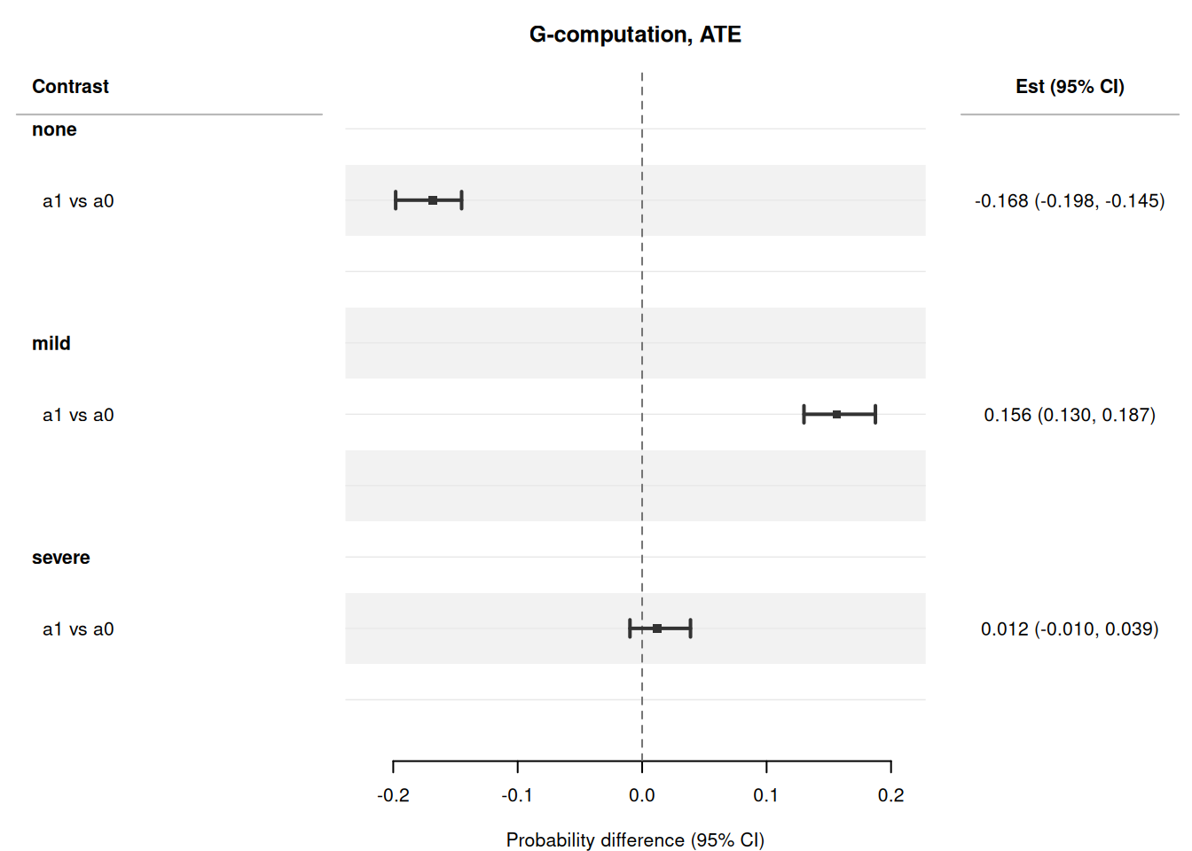
Within each intervention the class probabilities sum to 1, and the
per-class risk differences sum to 0 --- moving treatment shifts mass
between outcome levels:
```{r}
tt(tidy(res_mn, which = "means"), digits = 3)
```
A forest plot facets by outcome class automatically:
```{r}
#| fig-height: 5
plot(res_mn, which = "contrasts")
```
The analytic sandwich (`variance_if_gcomp_multinom()`) standardises the same
per-class softmax marginal-mean gradient through the multinomial-logit
influence function. It matches the bootstrap up to Monte-Carlo error:
```{r}
res_mn_sw <- contrast(
  fit_mn,
  interventions = list(a1 = static(1), a0 = static(0)),
  reference = "a0",
  type = "difference",
  ci_method = "sandwich"
)
tt(tidy(res_mn_sw, which = "means"), digits = 3)
```
### Survey-weighted multinomial sandwich
With survey or external weights (`weights =`), the outcome `nnet::multinom`
is a weighted MLE. The analytic sandwich carries the weights through the
weighted multinomial bread, the score residual, the Channel-1
empirical-distribution term, and the softmax marginal-mean gradient, so
`ci_method = "sandwich"` works directly --- no bootstrap fallback needed:
```{r}
set.seed(21)
mn_df$sw <- runif(nrow(mn_df), 0.5, 2)
fit_mn_w <- causat(
  mn_df,
  outcome = "Y",
  treatment = "A",
  confounders = ~ L,
  model_fn = nnet::multinom,
  trace = FALSE,
  weights = mn_df$sw
)
res_mn_w <- contrast(
  fit_mn_w,
  interventions = list(a1 = static(1), a0 = static(0)),
  reference = "a0",
  type = "difference",
  ci_method = "sandwich"
)
tt(tidy(res_mn_w, which = "means"), digits = 3)
```
### IPCW multinomial sandwich
When the categorical outcome is missing-at-random given the covariates,
`censoring = "C", ipcw = TRUE` fits a censoring model and reweights the
multinomial g-computation by the inverse probability of being uncensored. The
analytic sandwich then adds the censoring model's estimation uncertainty to the
per-class influence function through two channels: an *indirect* path (the
weights feed the outcome model) and a *direct* path (the weights feed the
inverse-probability-weighted average). The direct term recovers the efficiency
gain from estimating the censoring model and cancels in contrasts, so reported
difference / ratio / odds-ratio standard errors are unaffected while the
per-class marginal-probability standard errors are exact.
```{r}
set.seed(7)
mn_df$Cens <- rbinom(nrow(mn_df), 1, plogis(-0.6 + 0.5 * mn_df$A + 0.7 * mn_df$L))
mn_df$Y_obs <- mn_df$Y
mn_df$Y_obs[mn_df$Cens == 1] <- NA
fit_mn_ipcw <- causat(
  mn_df,
  outcome = "Y_obs",
  treatment = "A",
  confounders = ~ L,
  model_fn = nnet::multinom,
  trace = FALSE,
  censoring = "Cens",
  ipcw = TRUE
)
res_mn_ipcw <- contrast(
  fit_mn_ipcw,
  interventions = list(a1 = static(1), a0 = static(0)),
  reference = "a0",
  type = "difference",
  ci_method = "sandwich"
)
tt(tidy(res_mn_ipcw, which = "means"), digits = 3)
```
## GLM with splines
For flexible confounder adjustment without the overhead of a full GAM, use
`splines::ns()` (natural cubic splines) directly in the formula. This keeps
the model as a plain `glm`, so the analytic sandwich path fires --- unlike
GAM, no `mgcv` dependency is needed.
```{r}
fit_spline <- causat(
nhefs,
outcome = "wt82_71",
treatment = "qsmk",
confounders = ~ sex + splines::ns(age, 3) + race + factor(education) +
splines::ns(smokeintensity, 3) + splines::ns(smokeyrs, 3) +
factor(exercise) + factor(active) + splines::ns(wt71, 3),
censoring = "censored",
model_fn = stats::glm
)
res_spline <- contrast(
fit_spline,
interventions = list(quit = static(1), continue = static(0)),
reference = "continue",
ci_method = "sandwich"
)
res_spline
```
## GAM model via model_fn
Pass `mgcv::gam` instead of `stats::glm` for flexible nonlinear confounder
adjustment using splines.
```{r}
fit_gam <- causat(
nhefs,
outcome = "wt82_71",
treatment = "qsmk",
confounders = ~ sex + s(age) + race + factor(education) +
s(smokeintensity) + s(smokeyrs) + factor(exercise) +
factor(active) + s(wt71),
censoring = "censored",
model_fn = mgcv::gam
)
res_gam <- contrast(
fit_gam,
interventions = list(quit = static(1), continue = static(0)),
reference = "continue",
ci_method = "sandwich"
)
res_gam
```
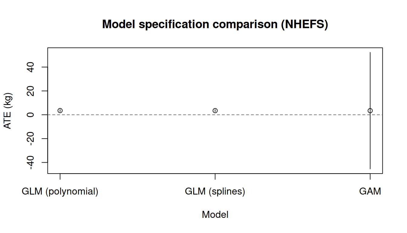
::: {.callout-note}
## GAM sandwich SEs can be larger than GLM SEs
The sandwich variance for GAMs uses the penalised Bayesian covariance
(`model$Vp`) as the bread inverse, which accounts for the smoothing
penalty. This can produce noticeably larger SEs than GLM-based models
(polynomial or spline), especially when the effective degrees of freedom
are high relative to the sample size. If the GAM SE looks disproportionately
large, consider using bootstrap inference (`ci_method = "bootstrap"`) or
switching to a GLM with `splines::ns()` terms, which stays on the standard
(unpenalised) analytic sandwich path.
:::
::: {.callout-warning}
## Machine learning outcome models require debiased estimation
causatr's `model_fn` argument accepts any GLM or GAM, but **not** machine
learning models (random forests, gradient boosting, neural networks). Two
reasons:
1. **Bias.** Plug-in ML predictions for the g-formula are biased at
$\sqrt{n}$ rate due to overfitting (regularisation bias / Dorn bias).
Consistent estimation requires cross-fitting + a bias-correction step
(one-step estimator, TMLE, or SDR), which causatr does not implement.
2. **Variance.** The sandwich variance estimator requires the parametric
likelihood score of the outcome model. ML models do not have one, so
causatr cannot compute standard errors.
If you need flexible (nonparametric) outcome models, use the
[`lmtp`](https://cran.r-project.org/package=lmtp) package, which
implements TMLE and SDR with Super Learner stacks and supports the same
intervention types (`shift`, `ipsi`, etc.). See @hernan_whatif, Ch. 18
and @vdl2011targeted for the theory behind debiased ML.
:::
### Comparing model specifications
All three approaches --- standard GLM with polynomial terms, GLM with natural
splines, and GAM --- target the same causal parameter. Differences in point
estimates reflect model flexibility; all three should agree closely when the
outcome model is correctly specified.
```{r}
#| fig-width: 7
#| fig-height: 4
#| fig-alt: "Forest plot comparing ATE estimates from GLM (polynomial), GLM (splines), and GAM model specifications."
model_comp <- data.frame(
  Model = c("GLM (polynomial)", "GLM (splines)", "GAM"),
  Estimate = c(
    res_ate_sw$contrasts$estimate[1],
    res_spline$contrasts$estimate[1],
    res_gam$contrasts$estimate[1]
  ),
  SE = c(
    res_ate_sw$contrasts$se[1],
    res_spline$contrasts$se[1],
    res_gam$contrasts$se[1]
  ),
  CI_lower = c(
    res_ate_sw$contrasts$ci_lower[1],
    res_spline$contrasts$ci_lower[1],
    res_gam$contrasts$ci_lower[1]
  ),
  CI_upper = c(
    res_ate_sw$contrasts$ci_upper[1],
    res_spline$contrasts$ci_upper[1],
    res_gam$contrasts$ci_upper[1]
  )
)

tt(model_comp, digits = 3)
```
```{r}
#| fig-width: 7
#| fig-height: 4
#| fig-alt: "Forest plot comparing ATE estimates from three model specifications."
tinyplot(
  Estimate ~ Model,
  data = model_comp,
  type = "pointrange",
  ymin = model_comp$CI_lower,
  ymax = model_comp$CI_upper,
  ylab = "ATE (kg)",
  main = "Model specification comparison (NHEFS)"
)
abline(h = 0, lty = 2, col = "grey40")
```
## Stochastic interventions
`stochastic()` defines a randomised intervention where the counterfactual
treatment for each individual is drawn from a user-supplied distribution. The
g-formula evaluates $E[Y^g]$ via Monte Carlo integration: for each of `n_mc`
draws, the sampler assigns counterfactual treatments, the outcome model
predicts, and the predictions are averaged across draws.
Stochastic interventions are only supported under g-computation (point and
longitudinal). See `vignette("interventions")` for a full comparison of
intervention types and estimator compatibility.
### Binary treatment: covariate-dependent randomisation
Assign quitting with a probability that depends on baseline smoking intensity
(heavier smokers are more likely to be assigned to quit):
```{r}
set.seed(42)
res_stoch <- contrast(
fit_gc,
interventions = list(
random_quit = stochastic(
\(data, trt) rbinom(nrow(data), 1,
plogis(-1 + 0.05 * data$smokeintensity)),
n_mc = 200L
),
all_quit = static(1)
),
reference = "all_quit",
type = "difference"
)
res_stoch
```
The stochastic policy's marginal mean is between the "all quit" and "no one
quits" extremes: heavier smokers are more likely to quit, but no one is forced.
### Continuous treatment: random shift
Rather than a fixed `shift(-10)`, add a random perturbation to each person's
smoking intensity:
```{r}
set.seed(42)
fit_cont_stoch <- causat(
nhefs_complete,
outcome = "wt82_71",
treatment = "smokeintensity",
confounders = ~ sex + age + I(age^2) + race + factor(education) +
smokeyrs + I(smokeyrs^2) + factor(exercise) + factor(active) +
wt71 + I(wt71^2),
model_fn = stats::glm
)
res_stoch_cont <- contrast(
fit_cont_stoch,
interventions = list(
noisy_reduce = stochastic(
\(data, trt) pmax(0, trt + rnorm(length(trt), mean = -5, sd = 2)),
n_mc = 200L
),
observed = NULL
),
reference = "observed",
type = "difference"
)
res_stoch_cont
```
::: {.callout-tip}
**Choosing `n_mc`**: 100--500 is typical. The sandwich SE accounts for the MC
draws used at estimation time, so there is no need to inflate `n_mc` just for
inference. If point estimates visibly change when you re-run with a different
seed, increase `n_mc`.
:::
## Summary of covered combinations
**Legend.** ✅ covered and truth-pinned in tests · 🟡 smoke test only ·
⛔ rejected with an informative error.
| Treatment | Outcome | Intervention | Estimand | Contrast | Inference | Weights | Status |
|---|---|---|---|---|---|---|---|
| Binary | Continuous (gaussian, GLM) | Static | ATE | Difference | Sandwich | none | ✅ |
| Binary | Continuous (gaussian, GLM) | Static | ATE | Difference | Bootstrap | none | ✅ |
| Binary | Continuous (gaussian, GLM) | Static | ATT | Difference | Sandwich | none | ✅ |
| Binary | Continuous (gaussian, GLM) | Static | ATC | Difference | Sandwich | none | ✅ |
| Binary | Continuous (gaussian, GLM) | Static | Subset | Difference | Sandwich | none | ✅ |
| Binary | Continuous (gaussian, GLM) | Static | ATE (by sex, `A:sex` in model) | Difference | Sandwich | none | ✅ |
| Binary | Continuous (gaussian, GLM) | Dynamic | ATE | Difference | Sandwich | none | ✅ |
| Binary | Continuous (gaussian, GLM) | Static | ATE | Difference | Sandwich | survey | ✅ |
| Binary | Continuous (gaussian, GAM) | Static | ATE | Difference | Sandwich | none | ✅ |
| Binary | Binary (binomial, GLM) | Static | ATE | Difference | Sandwich | none | ✅ |
| Binary | Binary (binomial, GLM) | Static | ATE | Difference | Bootstrap | none | ✅ |
| Binary | Binary (binomial, GLM) | Static | ATE | Ratio | Sandwich | none | ✅ |
| Binary | Binary (binomial, GLM) | Static | ATE | OR | Sandwich | none | ✅ |
| Binary | Count (poisson, GLM) | Static | ATE | Ratio | Sandwich | none | ✅ |
| Binary | Positive continuous (Gamma, GLM) | Static | ATE | Ratio | Sandwich | none | ✅ |
| Binary | Binary (quasibinomial, GLM) | Static | ATE | Difference | Sandwich | none | ✅ |
| Binary | Continuous (gaussian, GLM+splines) | Static | ATE | Difference | Sandwich | none | ✅ |
| Continuous | Continuous (gaussian, GLM) | Static | ATE | Difference | Sandwich | none | ✅ |
| Continuous | Continuous (gaussian, GLM) | Shift | ATE | Difference | Sandwich | none | ✅ |
| Continuous | Continuous (gaussian, GLM) | Scale | ATE | Difference | Sandwich | none | ✅ |
| Continuous | Continuous (gaussian, GLM) | Threshold | ATE | Difference | Sandwich | none | ✅ |
| Continuous | Continuous (gaussian, GLM) | Dynamic | ATE | Difference | Sandwich | none | ✅ |
| Continuous | Continuous (gaussian, GLM) | Shift | ATE | Difference | Bootstrap | none | ✅ |
| Categorical (k>2) | Continuous (gaussian, GLM) | Static | ATE | Difference | Sandwich | none | ✅ |
| Multivariate | Continuous (gaussian, GLM) | Joint static | ATE | Difference | Sandwich | none | ✅ |
| Binary | Continuous (gaussian, GLM) | Stochastic | ATE | Difference | Sandwich | none | ✅ |
| Continuous | Continuous (gaussian, GLM) | Stochastic | ATE | Difference | Sandwich | none | ✅ |
| Binary | Count (NB, `MASS::glm.nb`) | Static | ATE | Ratio | Sandwich | none | ✅ |
| Binary | Proportion (beta, `betareg::betareg`) | Static | ATE | Difference | Sandwich | none | ✅ |
See `FEATURE_COVERAGE_MATRIX.md`
for the authoritative coverage status of every method × treatment × outcome
× intervention × variance combination, including censoring and the numeric
two-tier variance fallback for custom `model_fn` choices.
## References
::: {#refs}
:::