---
title: "Inverse probability weighting with causatr"
code-fold: show
code-tools: true
vignette: >
%\VignetteIndexEntry{Inverse probability weighting with causatr}
%\VignetteEngine{quarto::html}
%\VignetteEncoding{UTF-8}
bibliography: references.bib
---
```{r}
#| include: false
knitr::opts_chunk$set(collapse = TRUE, comment = "#>")
```
Inverse probability weighting (IPW) estimates causal effects by reweighting
the observed data so that the distribution of confounders is balanced across
treatment groups. causatr ships a self-contained density-ratio engine that
fits the conditional treatment density via the user's `propensity_model_fn`
(default `stats::glm`) and builds per-intervention Hájek weights for an
intercept-only marginal structural model (MSM) refit inside `contrast()`.
This vignette demonstrates IPW in causatr using the NHEFS dataset from
@hernan_whatif, covering every supported combination of treatment type,
outcome type, contrast scale, and inference method for time-fixed treatments.
For non-static interventions (shift, scale, dynamic, IPSI), see
`vignette("interventions")`.
**Note:** IPW and matching support effect modification via `A:modifier`
terms in `confounders`. IPW expands the per-intervention MSM to include
modifier main effects (`Y ~ 1 + modifier`); matching expands to a
saturated MSM (`Y ~ A + modifier + A:modifier`). Use `by = "modifier"`
in `contrast()` to obtain stratum-specific estimates.
## Setup
The examples in this vignette use the **NHEFS** (National Health and
Nutrition Examination Survey --- Epidemiologic Follow-up Study) dataset,
the running example in @hernan_whatif. The assumed causal
structure is:
- **Treatment ($A$):** `qsmk` --- quit smoking between 1971 and 1982 (binary: 0/1).
- **Outcome ($Y$):** `wt82_71` --- weight change in kg over the same period
(continuous). A derived binary version, `gained_weight` ($\mathbf{1}\{Y > 0\}$),
is used in the binary outcome sections.
- **Confounders ($L$):** sex, age, race, education, smoking intensity
(cigarettes/day), years smoked, exercise, physical activity, and baseline
weight. These jointly affect both the probability of quitting and the
subsequent weight change.
Structural causal model (assumed):
$$
\begin{aligned}
L &\sim F_L \\
A &\sim \text{Bernoulli}\!\bigl(\text{logit}^{-1}(\alpha_0 + \alpha_L^\top L)\bigr) \\
Y &= \beta_0 + \beta_A A + \beta_L^\top L + \beta_{AL}^\top (A \cdot L) + \varepsilon,
\quad \varepsilon \sim N(0, \sigma^2)
\end{aligned}
$$
The confounders $L$ are common causes of $A$ and $Y$; adjusting for $L$
blocks all backdoor paths, identifying $\mathbb{E}[Y^a]$ via the
Horvitz--Thompson reweighting estimator. IPW models the treatment
mechanism $P(A \mid L)$ directly and reweights outcomes to remove
confounding, rather than modelling $E[Y \mid A, L]$ as g-computation does.
```{r}
#| message: false
library(causatr)
library(tinytable)
library(tinyplot)

data("nhefs")

nhefs_complete <- nhefs[!is.na(nhefs$wt82_71) & !is.na(nhefs$education), ]

nhefs_complete$gained_weight <- as.integer(nhefs_complete$wt82_71 > 0)

nhefs_complete$sex <- factor(
  nhefs_complete$sex,
  levels = 0:1,
  labels = c("Male", "Female")
)
```
## Binary treatment, continuous outcome
This replicates the IPW analysis from @hernan_whatif, Ch. 12: the
average causal effect of quitting smoking (`qsmk`) on weight change
(`wt82_71`). By default, `confounders` specifies the same covariate
set for the propensity model. Use `confounders_treatment` to specify
a different set for the treatment model when needed (e.g. for AIPW
double robustness).
### ATE with sandwich SE
```{r}
fit_ipw <- causat(
  nhefs_complete,
  outcome = "wt82_71",
  treatment = "qsmk",
  confounders = ~ sex + age + I(age^2) + race + factor(education) +
    smokeintensity + I(smokeintensity^2) + smokeyrs + I(smokeyrs^2) +
    factor(exercise) + factor(active) + wt71 + I(wt71^2),
  estimator = "ipw",
  estimand = "ATE",
  model_fn = stats::glm,
  propensity_model_fn = stats::glm
)

res_ate_sw <- contrast(
  fit_ipw,
  interventions = list(quit = static(1), continue = static(0)),
  reference = "continue",
  type = "difference",
  ci_method = "sandwich"
)
res_ate_sw
```
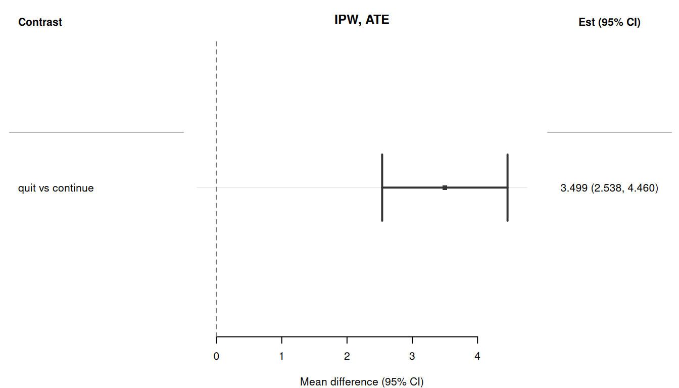
The book reports an IPW estimate of ATE $\approx$ 3.4 kg (95% CI: 2.4, 4.5).
### ATE with bootstrap SE
```{r}
res_ate_bs <- contrast(
  fit_ipw,
  interventions = list(quit = static(1), continue = static(0)),
  reference = "continue",
  type = "difference",
  ci_method = "bootstrap",
  n_boot = 50L
)
res_ate_bs
```
### ATT estimand
For IPW, the estimand is fixed at fitting time because it determines the
weights. To estimate the ATT, refit with `estimand = "ATT"`.
```{r}
fit_ipw_att <- causat(
  nhefs_complete,
  outcome = "wt82_71",
  treatment = "qsmk",
  confounders = ~ sex + age + I(age^2) + race + factor(education) +
    smokeintensity + I(smokeintensity^2) + smokeyrs + I(smokeyrs^2) +
    factor(exercise) + factor(active) + wt71 + I(wt71^2),
  estimator = "ipw",
  estimand = "ATT",
  model_fn = stats::glm,
  propensity_model_fn = stats::glm
)

res_att <- contrast(
  fit_ipw_att,
  interventions = list(quit = static(1), continue = static(0)),
  reference = "continue",
  type = "difference",
  ci_method = "sandwich"
)
res_att
```
### ATC estimand
```{r}
fit_ipw_atc <- causat(
  nhefs_complete,
  outcome = "wt82_71",
  treatment = "qsmk",
  confounders = ~ sex + age + I(age^2) + race + factor(education) +
    smokeintensity + I(smokeintensity^2) + smokeyrs + I(smokeyrs^2) +
    factor(exercise) + factor(active) + wt71 + I(wt71^2),
  estimator = "ipw",
  estimand = "ATC",
  model_fn = stats::glm,
  propensity_model_fn = stats::glm
)

res_atc <- contrast(
  fit_ipw_atc,
  interventions = list(quit = static(1), continue = static(0)),
  reference = "continue",
  type = "difference",
  ci_method = "sandwich"
)
res_atc
```
### ATT with bootstrap SE
```{r}
res_att_bs <- contrast(
  fit_ipw_att,
  interventions = list(quit = static(1), continue = static(0)),
  reference = "continue",
  type = "difference",
  ci_method = "bootstrap",
  n_boot = 50L
)
res_att_bs
```
### Extracting results programmatically
```{r}
coef(res_ate_sw)
confint(res_ate_sw)
vcov(res_ate_sw)
tidy(res_ate_sw)
glance(res_ate_sw)
```
## Binary treatment, binary outcome
Using the `gained_weight` indicator as a binary outcome. The IPW engine
refits an intercept-only weighted MSM per intervention; `contrast()` computes
marginal risks and derives contrasts via the unified influence-function
variance engine (`variance_if()`), which for IPW uses
`compute_ipw_if_self_contained_one()` to build the per-individual IF on the
stacked propensity + MSM M-estimation system.
### Risk difference (sandwich)
```{r}
fit_ipw_bin <- causat(
  nhefs_complete,
  outcome = "gained_weight",
  treatment = "qsmk",
  confounders = ~ sex + age + I(age^2) + race + factor(education) +
    smokeintensity + I(smokeintensity^2) + smokeyrs + I(smokeyrs^2) +
    factor(exercise) + factor(active) + wt71 + I(wt71^2),
  estimator = "ipw",
  model_fn = stats::glm,
  propensity_model_fn = stats::glm
)

res_rd <- contrast(
  fit_ipw_bin,
  interventions = list(quit = static(1), continue = static(0)),
  reference = "continue",
  type = "difference",
  ci_method = "sandwich"
)
res_rd
```
### Risk difference (bootstrap)
```{r}
res_rd_bs <- contrast(
  fit_ipw_bin,
  interventions = list(quit = static(1), continue = static(0)),
  reference = "continue",
  type = "difference",
  ci_method = "bootstrap",
  n_boot = 50L
)
res_rd_bs
```
### Risk ratio
```{r}
res_rr <- contrast(
  fit_ipw_bin,
  interventions = list(quit = static(1), continue = static(0)),
  reference = "continue",
  type = "ratio",
  ci_method = "sandwich"
)
res_rr
```
### Odds ratio
```{r}
res_or <- contrast(
  fit_ipw_bin,
  interventions = list(quit = static(1), continue = static(0)),
  reference = "continue",
  type = "or",
  ci_method = "sandwich"
)
res_or
```
### Risk ratio (bootstrap)
```{r}
res_rr_bs <- contrast(
  fit_ipw_bin,
  interventions = list(quit = static(1), continue = static(0)),
  reference = "continue",
  type = "ratio",
  ci_method = "bootstrap",
  n_boot = 50L
)
res_rr_bs
```
## Parallel bootstrap
Bootstrap replicates can be parallelised by passing `parallel` and `ncpus`
straight through to `boot::boot()`:
```{r}
#| eval: false
res_par <- contrast(
  fit_ipw,
  interventions = list(quit = static(1), continue = static(0)),
  reference = "continue",
  ci_method = "bootstrap",
  n_boot = 200L,
  parallel = "multicore",  # or "snow" on Windows
  ncpus = 4L
)
```
These default to `getOption("boot.parallel", "no")` and
`getOption("boot.ncpus", 1L)`, so a session-wide
`options(boot.parallel = "multicore", boot.ncpus = 4L)` flips parallelism
on for every `contrast()` call without per-call plumbing.
## Dynamic intervention (binary treatment)
A `dynamic()` intervention assigns each individual to a treatment value
based on their covariates. Under IPW, dynamic rules on binary treatment
use Horwitz--Thompson indicator weights: $w_i = \mathbb{1}\{A_i = d(L_i)\} / f(d(L_i) \mid L_i)$.
```{r}
rule <- function(data, trt) {
  ifelse(data$smokeintensity > 20, 1L, 0L)
}

res_dyn <- contrast(
  fit_ipw,
  interventions = list(
    targeted = dynamic(rule),
    all_quit = static(1)
  ),
  reference = "all_quit",
  type = "difference"
)
res_dyn
```
Heavy smokers (> 20 cigs/day) are assigned to quit, others are left
untreated. The contrast with `static(1)` (all quit) tells us how
much is lost by targeting only heavy smokers.
```{r}
tt(tidy(res_dyn), digits = 3)
```
## IPSI --- incremental propensity score intervention
`ipsi(delta)` multiplies each individual's odds of treatment by `delta`
[@kennedy2019ipsi]. It is a smooth stochastic intervention that avoids
positivity violations --- no one is forced to a treatment value they
would never take.
```{r}
res_ipsi <- contrast(
  fit_ipw,
  interventions = list(
    double_odds = ipsi(2),
    observed = NULL
  ),
  reference = "observed",
  type = "difference"
)
res_ipsi
```
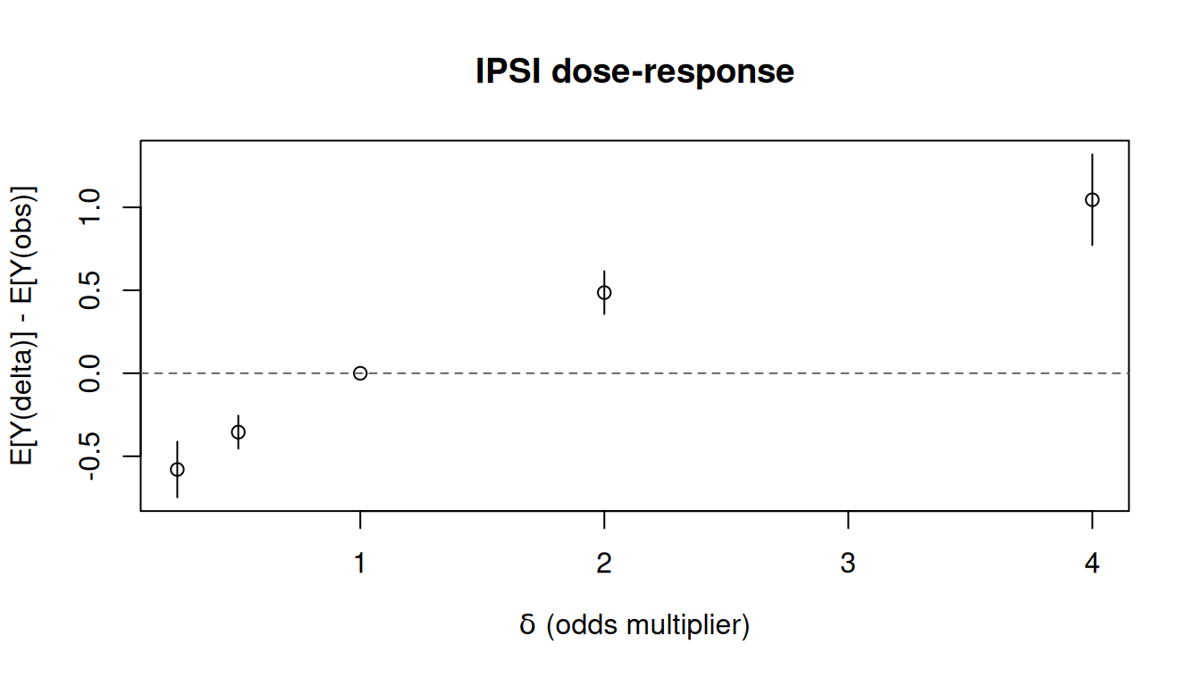
Varying `delta` traces out a dose--response curve:
```{r}
#| fig-width: 7
#| fig-height: 4
#| fig-alt: "IPSI dose-response curve showing the effect of varying the odds multiplier delta."
deltas <- c(0.25, 0.5, 1, 2, 4)
ipsi_results <- lapply(deltas, function(d) {
  r <- contrast(
    fit_ipw,
    interventions = list(ipsi = ipsi(d), obs = NULL),
    reference = "obs",
    type = "difference"
  )
  data.frame(
    delta = d,
    estimate = r$contrasts$estimate[1],
    ci_lower = r$contrasts$ci_lower[1],
    ci_upper = r$contrasts$ci_upper[1]
  )
})
ipsi_df <- do.call(rbind, ipsi_results)

tinyplot(
  estimate ~ delta,
  data = ipsi_df,
  type = "pointrange",
  ymin = ipsi_df$ci_lower,
  ymax = ipsi_df$ci_upper,
  xlab = expression(delta ~ "(odds multiplier)"),
  ylab = "E[Y(delta)] - E[Y(obs)]",
  main = "IPSI dose-response"
)
abline(h = 0, lty = 2, col = "grey40")
```
At `delta = 1` the intervention equals the natural course, so the contrast
is zero. Values below 1 reduce the odds of treatment; values above 1
increase them.
## Categorical treatment (k > 2 levels)
The density-ratio engine auto-selects a multinomial propensity model (via
`nnet::multinom`) when the treatment is a factor or character column. The
per-intervention MSM is intercept-only, so `contrast()` computes any pairwise
difference against a user-chosen reference level.
**DGM.** A single confounder $L$ influences both the three-level categorical
treatment $A \in \{A, B, C\}$ and the outcome $Y$. Treatment assignment
follows a softmax (multinomial logistic) model with category A as the
reference level. The outcome is linear in the treatment indicators and $L$.
$$
\begin{aligned}
L &\sim N(0, 1) \\
P(A = k \mid L) &= \frac{\exp(\gamma_k L)}{\sum_{j} \exp(\gamma_j L)},
\quad \gamma_A = 0,\; \gamma_B = 0.5,\; \gamma_C = -0.3 \\
Y &= 2 + 1.5 \cdot \mathbf{1}\{A = B\} - 0.8 \cdot \mathbf{1}\{A = C\}
+ 0.5\, L + \varepsilon,
\quad \varepsilon \sim N(0, 1)
\end{aligned}
$$
True contrasts (vs. reference A): $\mathbb{E}[Y^B] - \mathbb{E}[Y^A] = 1.5$
and $\mathbb{E}[Y^C] - \mathbb{E}[Y^A] = -0.8$.
```{r}
set.seed(42)
n <- 2000
L <- rnorm(n)
probs <- exp(cbind(0, 0.5 * L, -0.3 * L))
probs <- probs / rowSums(probs)
A <- factor(
  apply(probs, 1, function(p) sample(c("A", "B", "C"), 1, prob = p)),
  levels = c("A", "B", "C")
)
Y <- 2 + (A == "B") * 1.5 + (A == "C") * -0.8 + 0.5 * L + rnorm(n)
cat_df <- data.frame(Y = Y, A = A, L = L)

fit_ipw_cat <- causat(
  cat_df,
  outcome = "Y",
  treatment = "A",
  confounders = ~ L,
  estimator = "ipw",
  model_fn = stats::glm,
  propensity_model_fn = nnet::multinom
)

res_ipw_cat <- contrast(
  fit_ipw_cat,
  interventions = list(
    arm_a = static("A"),
    arm_b = static("B"),
    arm_c = static("C")
  ),
  reference = "arm_a",
  type = "difference"
)
res_ipw_cat
```
## Continuous treatment (shift / scale MTPs)
For continuous treatments the engine fits a Gaussian treatment density model
and uses density-ratio weights for modified treatment policies. `static()`
interventions on continuous treatments are rejected (nobody is observed
exactly at the target value, so the HT indicator is zero almost surely).
Use `shift()` or `scale_by()` instead:
**DGM.** A single confounder $L$ drives both a continuous (Gaussian)
treatment $A$ and a continuous outcome $Y$. The treatment density
is $A \mid L \sim N(1 + 0.5\, L,\; 1)$ and the outcome is linear in
$A$ and $L$ with additive noise.
$$
\begin{aligned}
L &\sim N(0, 1) \\
A \mid L &\sim N(1 + 0.5\, L,\; 1) \\
Y &= 1 + 2\, A + L + \varepsilon, \quad \varepsilon \sim N(0, 1)
\end{aligned}
$$
Because $\partial Y / \partial A = 2$, a unit additive shift
$A \mapsto A + 1$ has true causal effect
$\mathbb{E}[Y(A + 1)] - \mathbb{E}[Y(A)] = 2$.
```{r}
set.seed(5)
n <- 2000
L <- rnorm(n)
A <- 1 + 0.5 * L + rnorm(n)
Y <- 1 + 2 * A + L + rnorm(n)
cont_df <- data.frame(Y = Y, A = A, L = L)

fit_ipw_cont <- causat(
  cont_df,
  outcome = "Y",
  treatment = "A",
  confounders = ~ L,
  estimator = "ipw",
  model_fn = stats::glm,
  propensity_model_fn = stats::glm
)

res_shift <- contrast(
  fit_ipw_cont,
  interventions = list(up1 = shift(1), observed = NULL),
  reference = "observed",
  type = "difference"
)
res_shift
res_scale <- contrast(
  fit_ipw_cont,
  interventions = list(doubled = scale_by(2), observed = NULL),
  reference = "observed",
  type = "difference"
)
res_scale
```
Structural truth: `E[Y(A+1)] - E[Y(A)] = 2` (the coefficient on `A`).
See `vignette("interventions")` for a full tour of shift, scale, dynamic,
and IPSI interventions with side-by-side g-comp and IPW examples.
## Count treatment (Poisson / negative binomial)
Integer-valued treatments --- dose levels, event counts, visit counts --- default
to a Gaussian treatment density, which works when the support is dense enough
that the Normal approximation is harmless (age in years, cigarettes/day). For
sparse count data (0--5 doses), the Gaussian pdf evaluates between integers that
carry zero probability, producing badly calibrated density ratios.
Pass `propensity_family = "poisson"` or `propensity_family = "negbin"` to opt
into a Poisson or negative binomial treatment density model:
**DGM.** A confounder $L$ affects both a Poisson-distributed count
treatment $A$ and a continuous outcome $Y$. The treatment is generated
from a log-linear Poisson model and the outcome is linear in $A$ and $L$.
$$
\begin{aligned}
L &\sim N(0, 1) \\
A \mid L &\sim \text{Poisson}\!\bigl(\exp(0.5\, L)\bigr) \\
Y &= 2 + 1.5\, A + L + \varepsilon, \quad \varepsilon \sim N(0, 1)
\end{aligned}
$$
Because $\partial Y / \partial A = 1.5$, a unit shift $A \mapsto A + 1$
has true causal effect $\mathbb{E}[Y(A + 1)] - \mathbb{E}[Y(A)] = 1.5$.
```{r}
set.seed(6)
n <- 3000
L <- rnorm(n)
A <- rpois(n, exp(0.5 * L))
Y <- 2 + 1.5 * A + L + rnorm(n)
count_df <- data.frame(Y = Y, A = A, L = L)

fit_pois <- causat(
  count_df,
  outcome = "Y",
  treatment = "A",
  confounders = ~ L,
  estimator = "ipw",
  propensity_family = "poisson",
  model_fn = stats::glm,
  propensity_model_fn = stats::glm
)

res_pois <- contrast(
  fit_pois,
  interventions = list(plus1 = shift(1), observed = NULL),
  reference = "observed",
  type = "difference"
)
res_pois
```
Structural truth: `E[Y(A+1)] - E[Y(A)] = 1.5`.
For negative binomial (which nests Poisson when theta is large), pass
`propensity_family = "negbin"`. `MASS::glm.nb` is auto-selected as the
propensity fitter:
```{r}
#| eval: !expr requireNamespace("MASS", quietly = TRUE)
fit_nb <- causat(
count_df,
outcome = "Y",
treatment = "A",
confounders = ~ L,
estimator = "ipw",
propensity_family = "negbin",
model_fn = stats::glm,
propensity_model_fn = MASS::glm.nb
)
res_nb <- contrast(
fit_nb,
interventions = list(plus1 = shift(1), observed = NULL),
reference = "observed",
type = "difference"
)
res_nb
```
`scale_by()` also works on count treatments, but with a stricter constraint:
the density ratio evaluates at `A / factor`, so `A / factor` must be a
non-negative integer for *every* observed value. In practice, this means
`scale_by()` on counts is only feasible when all observed counts are multiples
of the factor.
::: {.callout-important}
## Integer constraints on count interventions
Only `shift()` with an integer delta and `scale_by()` where `A / factor` is
integer for every observation are allowed. `static()`, `dynamic()`,
`threshold()`, and `ipsi()` are rejected because the count pmf is zero at
non-integer arguments and the HT indicator / IPSI closed form require
binary structure. Use `estimator = "gcomp"` for those intervention types on
count data.
:::
## GAM propensity model
Pass `propensity_model_fn = mgcv::gam` to use a GAM for the treatment
density model while keeping the default `stats::glm` for the outcome MSM:
```{r}
#| eval: !expr requireNamespace("mgcv", quietly = TRUE)
fit_gam_ps <- causat(
  nhefs_complete,
  outcome = "wt82_71",
  treatment = "qsmk",
  confounders = ~ sex + s(age) + race + factor(education) +
    s(smokeintensity) + s(smokeyrs) + factor(exercise) +
    factor(active) + s(wt71),
  estimator = "ipw",
  model_fn = stats::glm,
  propensity_model_fn = mgcv::gam
)

res_gam_ps <- contrast(
  fit_gam_ps,
  interventions = list(quit = static(1), continue = static(0)),
  reference = "continue",
  type = "difference"
)
res_gam_ps
```
## External (survey) weights
Pre-computed survey weights are passed via `weights =`; causatr validates
them via `check_weights()` and **multiplies** them element-wise with the
estimated density-ratio weights. The combined weight drives both the
per-intervention MSM fit and the influence-function sandwich variance.
**DGM.** A simple confounded binary treatment with a continuous outcome.
Random survey weights (independent of the data-generating process) are
attached to illustrate external weight handling.
$$
\begin{aligned}
L &\sim N(0, 1) \\
A \mid L &\sim \text{Bernoulli}\!\bigl(\text{logit}^{-1}(0.5\, L)\bigr) \\
Y &= 2 + 3\, A + 1.5\, L + \varepsilon, \quad \varepsilon \sim N(0, 1) \\
w_i &\stackrel{\text{iid}}{\sim} \text{Uniform}(0.5,\; 2.0)
\end{aligned}
$$
True ATE: $\mathbb{E}[Y^1] - \mathbb{E}[Y^0] = 3$.
```{r}
set.seed(6)
n <- 2000
L <- rnorm(n)
A <- rbinom(n, 1, plogis(0.5 * L))
Y <- 2 + 3 * A + 1.5 * L + rnorm(n)
w <- runif(n, 0.5, 2.0)
sv_df <- data.frame(Y = Y, A = A, L = L)

fit_ipw_sv <- causat(
  sv_df,
  outcome = "Y",
  treatment = "A",
  confounders = ~ L,
  estimator = "ipw",
  weights = w,
  model_fn = stats::glm,
  propensity_model_fn = stats::glm
)

res_ipw_sv <- contrast(
  fit_ipw_sv,
  interventions = list(a1 = static(1), a0 = static(0)),
  reference = "a0",
  type = "difference"
)
res_ipw_sv
```
### Direct `survey::svydesign` integration
`causat(weights = ...)` also accepts a `survey::svydesign` object
directly — `stats::weights(design)` is used to extract the sampling
weights and the design's first-stage PSU is auto-adopted as the
contrast-time cluster (see below). Explicit `cluster =` overrides the
adoption; single-PSU designs (`svydesign(ids = ~1, ...)`) propagate
only the weights.
```{r}
#| eval: false
library(survey)
des <- svydesign(ids = ~psu, weights = ~pw, data = d)
fit <- causat(d, outcome = "Y", treatment = "A",
              confounders = ~ L, estimator = "ipw",
              weights = des,
              model_fn = stats::glm, propensity_model_fn = stats::glm)
```
## Cluster-robust sandwich
For design clusters (site, household, PSU, repeated measures) the IPW
sandwich should account for within-cluster comovement of the
per-individual IFs. `causat(cluster = "col")` preserves the column
through `prepare_data()` and stashes it on the fit; `contrast()`
defaults to that cluster and runs the sum-within-cluster-then-square
IF aggregation. Numerically equivalent to `sandwich::vcovCL(type =
"HC0")` on the final MSM-fit → predict-then-average step, up to the
usual $G/(G-1)$ small-cluster factor.
```{r}
#| eval: false
fit_cl <- causat(d, outcome = "Y", treatment = "A",
                 confounders = ~ L, estimator = "ipw",
                 cluster = "site",
                 model_fn = stats::glm, propensity_model_fn = stats::glm)
contrast(fit_cl, list(a1 = static(1), a0 = static(0)))
```
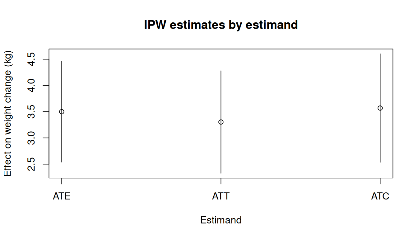
## Comparing estimands
```{r}
#| fig-width: 7
#| fig-height: 4
#| fig-alt: "Point estimates and confidence intervals for ATE, ATT, and ATC estimated by IPW."
est_df <- data.frame(
  estimand = c("ATE", "ATT", "ATC"),
  estimate = c(
    res_ate_sw$contrasts$estimate[1],
    res_att$contrasts$estimate[1],
    res_atc$contrasts$estimate[1]
  ),
  ci_lower = c(
    res_ate_sw$contrasts$ci_lower[1],
    res_att$contrasts$ci_lower[1],
    res_atc$contrasts$ci_lower[1]
  ),
  ci_upper = c(
    res_ate_sw$contrasts$ci_upper[1],
    res_att$contrasts$ci_upper[1],
    res_atc$contrasts$ci_upper[1]
  )
)

tinyplot(
  estimate ~ estimand,
  data = est_df,
  type = "pointrange",
  ymin = est_df$ci_lower,
  ymax = est_df$ci_upper,
  xlab = "Estimand",
  ylab = "Effect on weight change (kg)",
  main = "IPW estimates by estimand"
)
abline(h = 0, lty = 2, col = "grey40")
```
## Effect modification with `by`
When `confounders` includes an `A:modifier` interaction term, IPW expands
the per-intervention MSM from `Y ~ 1` to `Y ~ 1 + modifier`. The modifier
main effects let `predict()` return stratum-specific counterfactual means;
the treatment itself is still absorbed by the density-ratio weights. Use
`by = "modifier"` in `contrast()` to recover heterogeneous treatment effects.
Here we add a `qsmk:sex` interaction to examine how the effect of quitting
smoking on weight change differs by sex. The propensity model automatically
strips the interaction term (it only enters the MSM, not the treatment model).
```{r}
fit_ipw_hte <- causat(
  nhefs_complete,
  outcome = "wt82_71",
  treatment = "qsmk",
  confounders = ~ sex + age + I(age^2) + race + factor(education) +
    smokeintensity + I(smokeintensity^2) + smokeyrs + I(smokeyrs^2) +
    factor(exercise) + factor(active) + wt71 + I(wt71^2) +
    qsmk:sex,
  estimator = "ipw",
  model_fn = stats::glm,
  propensity_model_fn = stats::glm
)

res_ipw_by_sex <- contrast(
  fit_ipw_hte,
  interventions = list(quit = static(1), continue = static(0)),
  reference = "continue",
  type = "difference",
  ci_method = "sandwich",
  by = "sex"
)
res_ipw_by_sex
```
::: {.callout-note}
The `A:modifier` term does not enter the propensity model --- it would
create a post-treatment variable problem. `build_ps_formula()` strips
interaction terms involving the treatment automatically. The modifier
enters only the per-intervention MSM as a main effect, enabling
stratum-specific counterfactual mean estimation under the density-ratio
weights.
:::
## Tidy and glance
causatr results work with the broom ecosystem via `tidy()` and `glance()`:
```{r}
tidy(res_ate_sw)
glance(res_ate_sw)
```
## Forest plot
The `plot()` method produces a forest plot using the `forrest` package.
```{r}
#| fig-width: 7
#| fig-height: 4
#| fig-alt: "Forest plot of the IPW-estimated ATE of quitting smoking on weight change."
#| eval: !expr requireNamespace("forrest", quietly = TRUE)
plot(res_ate_sw)
```
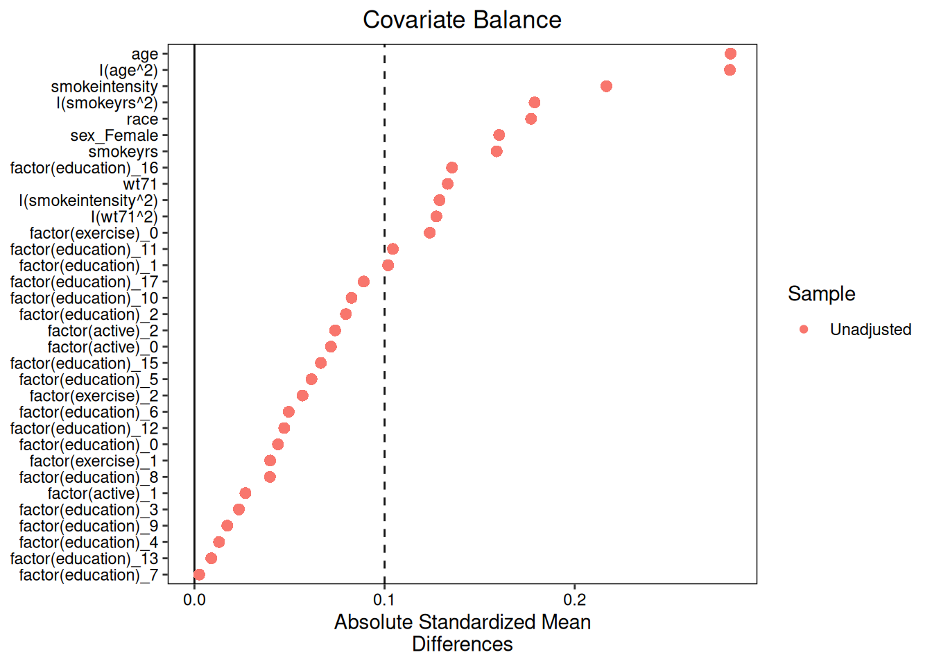
## Diagnostics
After fitting an IPW model, use `diagnose()` to assess positivity and
covariate balance. The balance diagnostics use
[cobalt](https://ngreifer.github.io/cobalt/) to compute standardised mean
differences (SMD) before and after weighting.
```{r}
diag <- diagnose(fit_ipw)
diag
```
### Love plot
A Love plot visualises covariate balance. Covariates with absolute SMD below
the threshold (dashed line at 0.1) are considered well-balanced.
```{r}
#| fig-width: 7
#| fig-height: 5
#| fig-alt: "Love plot showing covariate balance before and after IPW weighting."
plot(diag)
```
### Weight distribution
Extreme weights can inflate variance. The weight summary shows the effective
sample size (ESS) --- a large drop from the nominal sample size suggests
influential weights.
```{r}
diag$weights
```
## Weight truncation
When propensity models yield extreme density ratios --- due to near-positivity
violations, heavy confounding, or the cumulative product over many components or
time periods --- the resulting IPW estimator can be unstable with inflated
variance. The `trim` argument on `contrast()` winsorizes density-ratio weights
at a given quantile [@cole2008constructing; @spreafico2025positivity]. This is a
per-density-ratio operation applied *before* any multivariate or longitudinal
product, following the approach used internally by
[`lmtp`](https://cran.r-project.org/package=lmtp) (default 0.999).
```{r}
# Without truncation
res_raw <- contrast(
  fit_ipw, interventions = list(a1 = static(1), a0 = static(0)),
  ci_method = "sandwich"
)

# With truncation at the 99.9th percentile of the density ratio
res_trim <- contrast(
  fit_ipw, interventions = list(a1 = static(1), a0 = static(0)),
  ci_method = "sandwich", trim = 0.999
)
```
```{r}
#| echo: false
data.frame(
Truncation = c("None (trim = 1)", "trim = 0.999"),
Estimate = c(res_raw$contrasts$estimate, res_trim$contrasts$estimate),
SE = c(res_raw$contrasts$se, res_trim$contrasts$se)
) |>
tinytable::tt(digits = 4) |>
tinytable::format_tt(j = 2:3, digits = 3)
```
Truncation clips individual density ratios at their `trim`-th quantile
(upper-tail only). Key design choices:
- **Per-component, pre-product:** for multivariate IPW, each of the $K$
per-component ratios is truncated before the $\prod_k$ product. For
longitudinal IPW, per-period ratios are truncated before the cumulative
$\prod_t$ product.
- **Not applied to** sampling weights (transport) or IPCW weights (censoring)
--- those define the target population, not causal reweighting.
- **Sandwich SE** reflects the truncated weights: the threshold is held fixed at
the point estimate, so `numDeriv` perturbations evaluate the IF on the
truncated weight surface.
- **Bootstrap** recomputes the truncation threshold on each replicate, capturing
the full variance including the effect of truncation.
The default `trim = 1` applies no truncation and reproduces the standard IPW
estimator.
## Multivariate (joint) treatment
`estimator = "ipw"` accepts multiple treatment columns
`treatment = c("A1", "A2", ...)`. The engine factorises the joint conditional
density via the chain rule
$$f(A_1, \ldots, A_K \mid L) = \prod_{k=1}^{K} f_k(A_k \mid A_{1..k-1}, L)$$
and fits one univariate density model per component (sequential
factorisation). The joint density-ratio weight is the product of $K$
per-component ratios, with both numerator and denominator of the
$k$-th factor conditioning on **observed** upstream treatment
values --- only the $k$-th argument ($A_k$ vs $d_k^{-1}(A_k)$)
changes:
$$w_k(\alpha_k) = \frac{f_k\bigl(d_k^{-1}(A_k) \mid A_{1..k-1}^{\mathrm{obs}}, L; \alpha_k\bigr) \cdot |\mathrm{Jac}|}{f_k\bigl(A_k \mid A_{1..k-1}^{\mathrm{obs}}, L; \alpha_k\bigr)}.$$
This is the *sequential MTP* estimand of @diaz2023lmtp, the standard in
the causal-inference MTP literature.
Sandwich variance routes through a stacked propensity bread that is
block-diagonal across the $K$ models (each component is fit
independently), so the propensity correction sums $K$ single-model
corrections.
> **Multivariate gcomp implements a different estimand.** Multivariate
> gcomp computes
> $E[Y^d] = E\bigl\{E[Y \mid A_1 = d_1(A_1^{\mathrm{obs}}), A_2 = d_2(A_2^{\mathrm{obs}}), L]\bigr\}$
> under deterministic joint transformation: each individual's
> counterfactual is $(d_1(A_1^{\mathrm{obs}}), d_2(A_2^{\mathrm{obs}}))$,
> applied simultaneously per individual. For static-only
> interventions this coincides with the sequential MTP estimand; for
> non-static interventions on non-final components the two can differ
> by the upstream $\to$ downstream cross-dependence. Users who need
> gcomp-IPW triangulation on non-static multivariate policies should
> be aware of this estimand divergence.
The intervention is supplied as a *named list*, one entry per
treatment column, each entry a `causatr_intervention`:
```{r}
set.seed(42)
n <- 3000
L  <- rnorm(n)
A1 <- rbinom(n, 1, plogis(0.3 * L))
A2 <- rbinom(n, 1, plogis(-0.3 * L))
Y  <- 2 + 1.5 * A1 + 1.0 * A2 - 0.5 * L + rnorm(n)
df_mv <- data.frame(L = L, A1 = A1, A2 = A2, Y = Y)

fit_mv <- causat(
  df_mv, "Y", c("A1", "A2"), ~ L,
  estimator = "ipw",
  model_fn = stats::glm,
  propensity_model_fn = stats::glm
)
res_mv <- contrast(
  fit_mv,
  interventions = list(
    both    = list(A1 = static(1), A2 = static(1)),
    a1_only = list(A1 = static(1), A2 = static(0)),
    a2_only = list(A1 = static(0), A2 = static(1)),
    neither = list(A1 = static(0), A2 = static(0))
  ),
  reference = "neither"
)
tt(tidy(res_mv))
```
Truth on this DGP: $E[Y(1,1)] = 4.5$, $E[Y(0,0)] = 2.0$,
$\mathrm{ATE}(\text{both vs neither}) = 2.5$. Each component
intervention uses any of the regular constructors (`static()`,
`shift()`, `scale_by()`, `dynamic()`); IPSI in any component is
rejected because Kennedy's closed form has no joint analogue.
Component types can mix freely: binary × continuous, binary ×
categorical (via `nnet::multinom`), binary × Poisson / negative
binomial (via `propensity_family = c("", "poisson")` / `c("", "negbin")`),
continuous × continuous, and up to $K$-component combinations.
Effect modification `A_k:modifier` is supported — per-component
propensity formulas strip all treatment-touching terms and the MSM
expands to $Y \sim 1 + \mathrm{modifier\_main\_effects}$. Multivariate
matching remains rejected because `MatchIt` is binary-only.
### Stabilized weights
Pass `stabilize = "marginal"` to swap the per-component numerator for
a separately-fit model $g_k(A_k \mid A_{1..k-1})$ that drops $L$ from
the conditioning [@robins2000msmepi] (extended to the multivariate
case). The per-component weight becomes
$$
w_k^{s}(\alpha_k) = \frac{g_k\bigl(d_k^{-1}(A_k) \mid A_{1..k-1}\bigr) \cdot |\mathrm{Jac}|}{f_k(A_k \mid A_{1..k-1}, L; \alpha_k)}.
$$
```{r}
fit_mv_stab <- causat(
  df_mv, "Y", c("A1", "A2"), ~ L,
  estimator = "ipw", stabilize = "marginal",
  model_fn = stats::glm, propensity_model_fn = stats::glm
)
res_mv_stab <- contrast(
  fit_mv_stab,
  interventions = list(
    both    = list(A1 = static(1), A2 = static(1)),
    neither = list(A1 = static(0), A2 = static(0))
  ),
  reference = "neither"
)
tt(tidy(res_mv_stab))
```
Whether stabilization reduces or inflates the sandwich SE depends on
whether the marginal density of $A_k$ has lower variance than the
full-$L$ conditional — it's not universally beneficial, just a
common variance-reduction lever when $L$ strongly predicts $A_k$.
Numerator-model uncertainty is held fixed in the sandwich
(nuisance-fixed convention, same as $\sigma$ / $\theta$); bootstrap
refits both models and captures full variance.
### Mixed-type example
Mixed-type treatment (binary + continuous) just works:
```{r}
set.seed(7)
n <- 3000
L <- rnorm(n)
A1 <- rbinom(n, 1, 0.5)
A2 <- 5 + 0.5 * L + rnorm(n)
Y  <- 1 + 2 * A1 + 0.3 * A2 - 0.5 * L + rnorm(n)
df_mix <- data.frame(L = L, A1 = A1, A2 = A2, Y = Y)

fit_mix <- causat(
  df_mix, "Y", c("A1", "A2"), ~ L,
  estimator = "ipw",
  model_fn = stats::glm,
  propensity_model_fn = stats::glm
)
res_mix <- contrast(
  fit_mix,
  interventions = list(
    treat   = list(A1 = static(1), A2 = shift(-2)),
    control = list(A1 = static(0), A2 = shift(-2))
  ),
  reference = "control"
)
tt(tidy(res_mix))
```
The `A2` shift is applied uniformly under both arms, so the contrast
recovers the marginal `A1` effect (truth = 2).
### Multivariate + truncation
With $K$ components, the product weight $\prod_k w_k$ can grow rapidly.
`trim` truncates each per-component ratio *before* the product:
```{r}
res_mv_trim <- contrast(
  fit_mv,
  interventions = list(
    both    = list(A1 = static(1), A2 = static(1)),
    neither = list(A1 = static(0), A2 = static(0))
  ),
  reference = "neither",
  trim = 0.99
)
tt(tidy(res_mv_trim))
```
## Summary of covered combinations
**Legend.** ✅ covered and truth-pinned in tests · 🟡 smoke test only ·
⛔ rejected with an informative error.
| Treatment | Outcome | Intervention | Estimand | Contrast | Inference | Weights | Status |
|---|---|---|---|---|---|---|---|
| Binary | Continuous | Static | ATE | Difference | Sandwich | none | ✅ |
| Binary | Continuous | Static | ATE | Difference | Bootstrap | none | ✅ |
| Binary | Continuous | Static | ATT | Difference | Sandwich | none | ✅ |
| Binary | Continuous | Static | ATC | Difference | Sandwich | none | ✅ |
| Binary | Continuous | Static | ATT | Difference | Bootstrap | none | ✅ |
| Binary | Continuous | Static | ATE | Difference | Sandwich | survey | ✅ |
| Binary | Binary | Static | ATE | Difference | Sandwich | none | ✅ |
| Binary | Binary | Static | ATE | Difference | Bootstrap | none | ✅ |
| Binary | Binary | Static | ATE | Ratio | Sandwich | none | ✅ |
| Binary | Binary | Static | ATE | OR | Sandwich | none | ✅ |
| Binary | Binary | Static | ATE | Ratio | Bootstrap | none | ✅ |
| Binary | Continuous | Dynamic | ATE | Difference | Sandwich | none | ✅ |
| Binary | Continuous | IPSI($\delta$) | ATE | Difference | Sandwich | none | ✅ |
| Continuous | Continuous | Shift | ATE | Difference | Sandwich | none | ✅ |
| Continuous | Continuous | Scale | ATE | Difference | Sandwich | none | ✅ |
| Categorical (k>2) | Continuous | Static | ATE | Difference | Sandwich | none | ✅ |
| Categorical (k>2) | Continuous | Dynamic | ATE | Difference | Sandwich | none | 🟡 |
| Count (Poisson) | Continuous | Shift | ATE | Difference | Sandwich | none | ✅ |
| Count (NB) | Continuous | Shift | ATE | Difference | Sandwich | none | ✅ |
| Any | --- | Threshold | --- | --- | --- | --- | ⛔ (use gcomp) |
| Continuous | --- | Static | --- | --- | --- | --- | ⛔ (use shift/scale) |
| Continuous | --- | Dynamic | --- | --- | --- | --- | ⛔ (use shift/scale) |
| Binary | Gaussian | Static (with `A:modifier`) | ATE | Difference | Sandwich / Bootstrap | none | ✅ |
| Multi (bin × bin) | Gaussian | Static | ATE | Difference | Sandwich / Bootstrap | none | ✅ |
| Multi (bin × cont) | Gaussian | Static + Shift | ATE | Difference | Sandwich | none | ✅ |
| Multi (cont × cont) | Gaussian | Shift + Shift | ATE | Difference | Sandwich | none | ✅ (seq-MTP) |
| Multi (bin × bin) | Binary | Static | ATE | Diff / Ratio / OR | Sandwich | none | ✅ |
| Multi (3+ binary) | Gaussian | Static | ATE | Difference | Sandwich | none | ✅ |
| Multi (bin × bin) | Gaussian | Static (with `A_k:modifier`) | by-stratified | Difference | Sandwich | none | ✅ |
| Multi (bin × categorical) | Gaussian | Static | ATE | Difference | Sandwich | none | ✅ |
| Multi (bin × Poisson) | Gaussian | Static + Shift | ATE | Difference | Sandwich | none | ✅ |
| Multi (bin × negbin) | Gaussian | Static + Shift | ATE | Difference | Sandwich | none | ✅ |
| Multi (any) | --- | Any + `stabilize = "marginal"` | ATE | --- | Sandwich / Bootstrap | none | ✅ |
| Multi + IPSI component | --- | --- | --- | --- | --- | --- | ⛔ |
| Longitudinal | Continuous | Static / Shift / Scale / Dynamic | ATE | Difference | Sandwich / Bootstrap | none | ✅ (see `vignette("longitudinal")`) |
| Longitudinal | Continuous | Static + stabilize="marginal" | ATE | Difference | Sandwich | none | ✅ |
| Longitudinal | Any | IPSI | --- | --- | --- | --- | ⛔ (use point IPW) |
| Multivariate longitudinal | Continuous | Static / Shift | ATE | Difference | Sandwich / Bootstrap | none / marginal | ✅ (see `vignette("longitudinal")`) |
| Multivariate longitudinal | Gaussian | Static + EM (`A_k:modifier`) | by-stratified | Difference | Sandwich | none / marginal | ✅ vs ICE |
| Multivariate longitudinal | Any | IPSI component | --- | --- | --- | --- | ⛔ (use ICE) |
See `FEATURE_COVERAGE_MATRIX.md`
for the authoritative coverage status of every method × treatment × outcome
× intervention × variance combination.
## References
::: {#refs}
:::