Code
library(causatr)
library(tinytable)
library(tinyplot)Missing data is common in observational studies. causatr handles it differently depending on which variable is missing (outcome, treatment, or covariates) and which estimator is used. This vignette demonstrates the behaviour for each case and shows how to verify that your analysis is robust.
library(causatr)
library(tinytable)
library(tinyplot)We simulate a baseline dataset with known truth, then introduce missingness.
Data-generating mechanism. Two independent confounders \(L_1\) and \(L_2\) influence both a binary treatment \(A\) and a continuous outcome \(Y\). The treatment probability follows a logistic model in \(L_1\) and \(L_2\), and the outcome is linear in \(A\), \(L_1\), and \(L_2\) with additive Gaussian noise.
\[ \begin{aligned} L_1 &\sim \mathcal{N}(0, 1) \\ L_2 &\sim \mathcal{N}(0, 1) \\ A &\sim \text{Bernoulli}\bigl(\text{logit}^{-1}(0.3\,L_1 + 0.2\,L_2)\bigr) \\ Y &= 2 + 3\,A + 1.5\,L_1 + 0.8\,L_2 + \varepsilon, \quad \varepsilon \sim \mathcal{N}(0, 1) \end{aligned} \]
The treatment coefficient is 3 with no effect modification, so the true average treatment effect is \(\text{ATE} = E[Y^{a=1}] - E[Y^{a=0}] = 3\).
set.seed(42)
n <- 2000
L1 <- rnorm(n)
L2 <- rnorm(n)
A <- rbinom(n, 1, plogis(0.3 * L1 + 0.2 * L2))
Y <- 2 + 3 * A + 1.5 * L1 + 0.8 * L2 + rnorm(n)
df <- data.frame(Y = Y, A = A, L1 = L1, L2 = L2)When outcome values are missing completely at random (MCAR), the outcome model is fit on complete cases. contrast() predicts on all rows, then excludes rows with NA predictions from the target-population average. Under MCAR this is unbiased.
df_y_miss <- df
df_y_miss$Y[sample(n, round(0.15 * n))] <- NA

fit_y <- causat(
  df_y_miss,
  outcome = "Y",
  treatment = "A",
  confounders = ~ L1 + L2,
  model_fn = stats::glm
)

res_y <- contrast(
  fit_y,
  interventions = list(a1 = static(1), a0 = static(0)),
  reference = "a0",
  type = "difference",
  ci_method = "sandwich"
)
res_y
Estimator: gcomp · Estimand: ATE · Contrast: difference · CI method: sandwich · N: 2000
| intervention | estimate | se | ci_lower | ci_upper |
|---|---|---|---|---|
| a1 | 4.966 | 0.052 | 4.864 | 5.067 |
| a0 | 1.955 | 0.051 | 1.854 | 2.056 |
| comparison | estimate | se | ci_lower | ci_upper |
|---|---|---|---|---|
| a1 vs a0 | 3.011 | 0.049 | 2.914 | 3.107 |
The estimate remains close to 3 despite 15% missing outcomes.
fit_complete <- causat(
  df,
  outcome = "Y",
  treatment = "A",
  confounders = ~ L1 + L2,
  model_fn = stats::glm
)
res_complete <- contrast(
  fit_complete,
  interventions = list(a1 = static(1), a0 = static(0)),
  reference = "a0",
  type = "difference",
  ci_method = "sandwich"
)

comp_df <- data.frame(
  Analysis = c("Complete data", "15% outcome MCAR"),
  Estimate = c(res_complete$contrasts$estimate[1], res_y$contrasts$estimate[1]),
  SE = c(res_complete$contrasts$se[1], res_y$contrasts$se[1]),
  CI_lower = c(res_complete$contrasts$ci_lower[1], res_y$contrasts$ci_lower[1]),
  CI_upper = c(res_complete$contrasts$ci_upper[1], res_y$contrasts$ci_upper[1])
)
tt(comp_df, digits = 3)| Analysis | Estimate | SE | CI_lower | CI_upper |
|---|---|---|---|---|
| Complete data | 2.99 | 0.0456 | 2.91 | 3.08 |
| 15% outcome MCAR | 3.01 | 0.0492 | 2.91 | 3.11 |
The SE increases slightly with missing data (less information), but the point estimate stays on target.
IPW also handles missing outcomes. The treatment model is fit on the outcome-filtered subset (rows where Y is observed), and density-ratio weights are computed on that same subset.
fit_y_ipw <- causat(
  df_y_miss,
  outcome = "Y",
  treatment = "A",
  confounders = ~ L1 + L2,
  estimator = "ipw",
  model_fn = stats::glm,
  propensity_model_fn = stats::glm
)

res_y_ipw <- contrast(
  fit_y_ipw,
  interventions = list(a1 = static(1), a0 = static(0)),
  reference = "a0",
  type = "difference",
  ci_method = "sandwich"
)
res_y_ipw
Estimator: ipw · Estimand: ATE · Contrast: difference · CI method: sandwich · N: 2000
| intervention | estimate | se | ci_lower | ci_upper |
|---|---|---|---|---|
| a1 | 4.989 | 0.055 | 4.881 | 5.097 |
| a0 | 1.979 | 0.055 | 1.871 | 2.086 |
| comparison | estimate | se | ci_lower | ci_upper |
|---|---|---|---|---|
| a1 vs a0 | 3.01 | 0.049 | 2.913 | 3.107 |
Matching handles missing outcomes through MatchIt’s internal mechanisms. Rows with missing Y are excluded from the matched sample.
fit_y_match <- causat(
  df_y_miss,
  outcome = "Y",
  treatment = "A",
  confounders = ~ L1 + L2,
  estimator = "matching",
  estimand = "ATT"
)

res_y_match <- contrast(
  fit_y_match,
  interventions = list(a1 = static(1), a0 = static(0)),
  reference = "a0",
  type = "difference",
  ci_method = "sandwich"
)
res_y_match
Estimator: matching · Estimand: ATT · Contrast: difference · CI method: sandwich · N: 998
| intervention | estimate | se | ci_lower | ci_upper |
|---|---|---|---|---|
| a1 | 5.222 | 0.066 | 5.093 | 5.351 |
| a0 | 1.753 | 0.068 | 1.621 | 1.885 |
| comparison | estimate | se | ci_lower | ci_upper |
|---|---|---|---|---|
| a1 vs a0 | 3.469 | 0.055 | 3.362 | 3.577 |
methods_df <- data.frame(
  Method = c("G-comp", "IPW", "Matching (ATT)"),
  Estimate = c(
    res_y$contrasts$estimate[1],
    res_y_ipw$contrasts$estimate[1],
    res_y_match$contrasts$estimate[1]
  ),
  CI_lower = c(
    res_y$contrasts$ci_lower[1],
    res_y_ipw$contrasts$ci_lower[1],
    res_y_match$contrasts$ci_lower[1]
  ),
  CI_upper = c(
    res_y$contrasts$ci_upper[1],
    res_y_ipw$contrasts$ci_upper[1],
    res_y_match$contrasts$ci_upper[1]
  )
)

tinyplot(
  Estimate ~ Method,
  data = methods_df,
  type = "pointrange",
  ymin = methods_df$CI_lower,
  ymax = methods_df$CI_upper,
  ylab = "ATE estimate",
  main = "Three estimators under 15% outcome MCAR"
)
abline(h = 3, lty = 2, col = "grey40")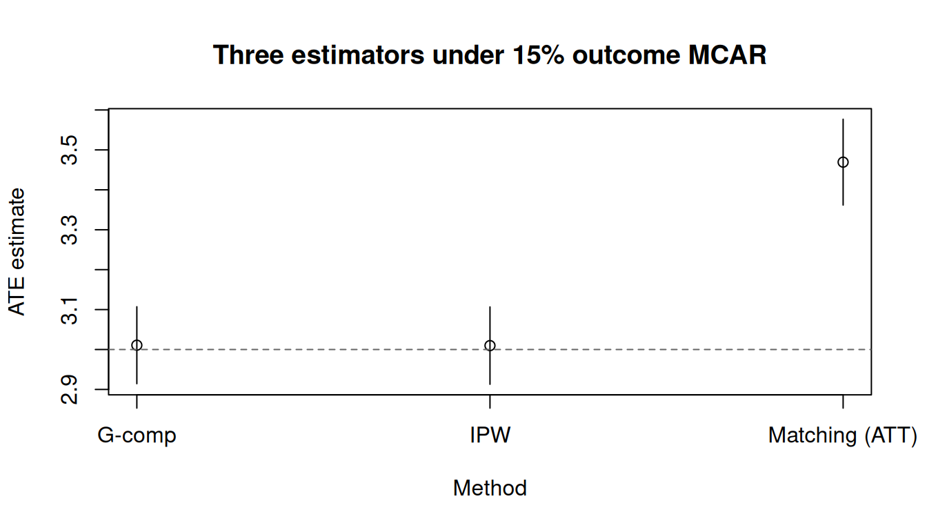
All three estimators recover the truth (dashed line at 3).
When covariates have missing values, glm(na.action = na.omit) drops those rows from the model fit. contrast() returns NA predictions for rows with missing covariates and excludes them from the target population.
df_l_miss <- df
df_l_miss$L1[sample(n, round(0.10 * n))] <- NA

fit_l <- causat(
  df_l_miss,
  outcome = "Y",
  treatment = "A",
  confounders = ~ L1 + L2,
  model_fn = stats::glm
)

res_l <- contrast(
  fit_l,
  interventions = list(a1 = static(1), a0 = static(0)),
  reference = "a0",
  type = "difference",
  ci_method = "sandwich"
)
#> 200 row(s) with NA predictions excluded from the target population.
res_l
Estimator: gcomp · Estimand: ATE · Contrast: difference · CI method: sandwich · N: 1800
| intervention | estimate | se | ci_lower | ci_upper |
|---|---|---|---|---|
| a1 | 4.995 | 0.052 | 4.893 | 5.096 |
| a0 | 2.006 | 0.052 | 1.903 | 2.108 |
| comparison | estimate | se | ci_lower | ci_upper |
|---|---|---|---|---|
| a1 vs a0 | 2.989 | 0.048 | 2.895 | 3.083 |
Under MCAR covariate missingness, the estimate is unbiased. Under MAR, the complete-case fit is biased — the missing rows are not a random sample of the data — and multiple imputation is needed. The next section walks through that workflow with causat_mice().
When covariates (or treatment) are missing at random (MAR) rather than completely at random, dropping the incomplete rows distorts the analysis: the observed subset is no longer representative. Multiple imputation (MI) fixes this by filling in the missing values from their predictive distribution several times, running the analysis on each completed dataset, and pooling. causatr’s causat_mice() is the analysis-and-pooling step: you impute upstream with mice::mice(), then hand the mids object to causat_mice(), which runs causat() + contrast() on every completed dataset and pools the results into a single causatr_result.
# Multiple imputation needs the mice package (a Suggested dependency). Every
# chunk in this section is guarded so the vignette still renders without it.
has_mice <- requireNamespace("mice", quietly = TRUE)
A MAR covariate. We simulate a confounder L whose missingness depends on the observed treatment A (so it is MAR, not MCAR) — L is recorded less often for the untreated. The true ATE is 3.
set.seed(2024)
n_mi <- 2000
L <- rnorm(n_mi)
A <- rbinom(n_mi, 1, plogis(0.5 * L))
Y <- 2 + 3 * A + 1.5 * L + rnorm(n_mi) # true ATE = 3
# L is observed more often among the treated -> missing more often among
# controls: missingness depends on the observed A (MAR, not MCAR).
R_L <- rbinom(n_mi, 1, plogis(0.6 + 0.7 * A))
df_full <- data.frame(Y = Y, A = A, L = L)
df_mar_l <- df_full
df_mar_l$L[R_L == 0] <- NA
round(mean(is.na(df_mar_l$L)), 2) # fraction of L missing
#> [1] 0.29
Helper to read a difference contrast as a signed magnitude with a symmetric interval (the reference direction is a display convention; the true effect is 3):
ate_row <- function(res, label) {
  e <- res$contrasts$estimate[1]
  half <- (res$contrasts$ci_upper[1] - res$contrasts$ci_lower[1]) / 2
  data.frame(Method = label, Estimate = abs(e),
             CI_lower = abs(e) - half, CI_upper = abs(e) + half)
}
Complete-case analysis discards the incomplete rows. A subtlety worth being honest about: under g-computation with a correctly specified outcome model, covariate missingness that depends only on modelled variables (here A) leaves the complete-case estimate approximately valid — so it will land near the truth below. But that is a fragile special case, not a general guarantee:
estimator = "ipw" or "matching", which abort on rows with a missing confounder, andMultiple imputation sidesteps all three by using every row and propagating the imputation uncertainty into the standard error.
cc_fit <- causat(df_mar_l, outcome = "Y", treatment = "A",
                 confounders = ~L, model_fn = stats::glm)
cc_res <- contrast(cc_fit, interventions = list(a1 = static(1), a0 = static(0)),
                   reference = "a0", type = "difference", ci_method = "sandwich")
#> 572 row(s) with NA predictions excluded from the target population.
cc_res
Estimator: gcomp · Estimand: ATE · Contrast: difference · CI method: sandwich · N: 1428
| intervention | estimate | se | ci_lower | ci_upper |
|---|---|---|---|---|
| a1 | 5.082 | 0.052 | 4.981 | 5.184 |
| a0 | 2.033 | 0.056 | 1.923 | 2.144 |
| comparison | estimate | se | ci_lower | ci_upper |
|---|---|---|---|---|
| a1 vs a0 | 3.049 | 0.056 | 2.94 | 3.158 |
Multiple imputation uses every row. Impute L with mice() (the default predictor matrix carries A and Y, which is exactly what we want — see the congeniality note below), then pool with causat_mice():
library(mice)
#>
#> Attaching package: 'mice'
#> The following object is masked from 'package:stats':
#>
#>     filter
#> The following objects are masked from 'package:base':
#>
#>     cbind, rbind
imp <- mice(df_mar_l, m = 20, printFlag = FALSE)

mi_res <- causat_mice(
  imp,
  outcome = "Y",
  treatment = "A",
  confounders = ~L,
  interventions = list(a1 = static(1), a0 = static(0)),
  estimator = "gcomp",
  type = "difference"
)
#> Warning: `model_fn` not specified; defaulting to `stats::glm`.
#> ℹ Set `model_fn` explicitly (e.g. `model_fn = stats::glm` or `model_fn = mgcv::gam`).
#> `model_fn` not specified; defaulting to `stats::glm`.
#> ℹ Set `model_fn` explicitly (e.g. `model_fn = stats::glm` or `model_fn = mgcv::gam`).
#> `model_fn` not specified; defaulting to `stats::glm`.
#> ℹ Set `model_fn` explicitly (e.g. `model_fn = stats::glm` or `model_fn = mgcv::gam`).
#> `model_fn` not specified; defaulting to `stats::glm`.
#> ℹ Set `model_fn` explicitly (e.g. `model_fn = stats::glm` or `model_fn = mgcv::gam`).
#> `model_fn` not specified; defaulting to `stats::glm`.
#> ℹ Set `model_fn` explicitly (e.g. `model_fn = stats::glm` or `model_fn = mgcv::gam`).
#> `model_fn` not specified; defaulting to `stats::glm`.
#> ℹ Set `model_fn` explicitly (e.g. `model_fn = stats::glm` or `model_fn = mgcv::gam`).
#> `model_fn` not specified; defaulting to `stats::glm`.
#> ℹ Set `model_fn` explicitly (e.g. `model_fn = stats::glm` or `model_fn = mgcv::gam`).
#> `model_fn` not specified; defaulting to `stats::glm`.
#> ℹ Set `model_fn` explicitly (e.g. `model_fn = stats::glm` or `model_fn = mgcv::gam`).
#> `model_fn` not specified; defaulting to `stats::glm`.
#> ℹ Set `model_fn` explicitly (e.g. `model_fn = stats::glm` or `model_fn = mgcv::gam`).
#> `model_fn` not specified; defaulting to `stats::glm`.
#> ℹ Set `model_fn` explicitly (e.g. `model_fn = stats::glm` or `model_fn = mgcv::gam`).
#> `model_fn` not specified; defaulting to `stats::glm`.
#> ℹ Set `model_fn` explicitly (e.g. `model_fn = stats::glm` or `model_fn = mgcv::gam`).
#> `model_fn` not specified; defaulting to `stats::glm`.
#> ℹ Set `model_fn` explicitly (e.g. `model_fn = stats::glm` or `model_fn = mgcv::gam`).
#> `model_fn` not specified; defaulting to `stats::glm`.
#> ℹ Set `model_fn` explicitly (e.g. `model_fn = stats::glm` or `model_fn = mgcv::gam`).
#> `model_fn` not specified; defaulting to `stats::glm`.
#> ℹ Set `model_fn` explicitly (e.g. `model_fn = stats::glm` or `model_fn = mgcv::gam`).
#> `model_fn` not specified; defaulting to `stats::glm`.
#> ℹ Set `model_fn` explicitly (e.g. `model_fn = stats::glm` or `model_fn = mgcv::gam`).
#> `model_fn` not specified; defaulting to `stats::glm`.
#> ℹ Set `model_fn` explicitly (e.g. `model_fn = stats::glm` or `model_fn = mgcv::gam`).
#> `model_fn` not specified; defaulting to `stats::glm`.
#> ℹ Set `model_fn` explicitly (e.g. `model_fn = stats::glm` or `model_fn = mgcv::gam`).
#> `model_fn` not specified; defaulting to `stats::glm`.
#> ℹ Set `model_fn` explicitly (e.g. `model_fn = stats::glm` or `model_fn = mgcv::gam`).
#> `model_fn` not specified; defaulting to `stats::glm`.
#> ℹ Set `model_fn` explicitly (e.g. `model_fn = stats::glm` or `model_fn = mgcv::gam`).
#> `model_fn` not specified; defaulting to `stats::glm`.
#> ℹ Set `model_fn` explicitly (e.g. `model_fn = stats::glm` or `model_fn = mgcv::gam`).
mi_res
Estimator: gcomp · Estimand: ATE · Contrast: difference · CI method: rubin · N: 2000
| intervention | estimate | se | ci_lower | ci_upper |
|---|---|---|---|---|
| a1 | 5.027 | 0.047 | 4.935 | 5.12 |
| a0 | 1.991 | 0.048 | 1.897 | 2.085 |
| comparison | estimate | se | ci_lower | ci_upper |
|---|---|---|---|---|
| a0 vs a1 | -3.037 | 0.053 | -3.141 | -2.932 |
The pooled standard error reflects both the within-imputation sampling variability and the between-imputation uncertainty, via Rubin’s (1987) rules with Barnard-Rubin (1999) degrees of freedom. The per-imputation diagnostics (including the fraction of missing information) live in the "mi_details" attribute:
attr(mi_res, "mi_details")$contrasts
#>         between      within       total      df       fmi
#>           <num>       <num>       <num>   <num>     <num>
#> 1: 0.0006324742 0.002169654 0.002833752 282.118 0.2397236
Be transparent about what MI does and does not buy here. Complete-case is valid in this design, and the two estimates agree closely — MI does not magically sharpen a valid analysis. It does still use the partially observed rows (so its interval is, if anything, a touch narrower than complete-case’s), and the fmi column reports how much information the missingness costs. The honest caveat runs the other way: MI is only as good as its imputation model. A misspecified imputation can bias the causal estimate worse than complete-case — we demonstrate exactly that below by dropping Y from the predictor matrix. MI’s decisive advantage, meanwhile, shows up when complete-case is biased — the next design.
Complete-case validity above hinged on L being missing as a function of A alone — a modelled covariate. Now make missingness depend on the outcome, and in opposite directions across treatment arms: among the treated L is recorded when Y is low, among controls when Y is high. The outcome regression conditions on covariates, not on its own selection, so the complete-case fit cannot undo this distortion and its ATE is badly biased. MI, which imputes L from (A, Y) over the whole sample, recovers the truth.
# Reusable complete-case (na.omit) + MI g-computation on a partially observed
# data frame, each summarised by ate_row().
cc_mi_gcomp <- function(dmar, m = 20) {
  ints <- list(a1 = static(1), a0 = static(0))
  cc <- contrast(
    causat(na.omit(dmar), outcome = "Y", treatment = "A",
           confounders = ~L, model_fn = stats::glm),
    interventions = ints, reference = "a0", ci_method = "sandwich"
  )
  imp_d <- mice(dmar, m = m, printFlag = FALSE)
  mi <- causat_mice(imp_d, outcome = "Y", treatment = "A", confounders = ~L,
                    interventions = ints, estimator = "gcomp")
  list(cc = cc, mi = mi)
}

set.seed(3)
n2 <- 4000
L2 <- rnorm(n2)
A2 <- rbinom(n2, 1, plogis(0.5 * L2))
Y2 <- 2 + 3 * A2 + 1.5 * L2 + rnorm(n2) # true ATE = 3
z2 <- (Y2 - mean(Y2)) / sd(Y2)
# Observe L with arm-flipped dependence on Y: MAR on (A, Y), unmodellable by a
# covariate-only outcome regression fit on complete cases.
R2 <- rbinom(n2, 1, plogis(1.0 + 1.8 * ifelse(A2 == 1, -z2, z2)))
df2_full <- data.frame(Y = Y2, A = A2, L = L2)
df2 <- df2_full
df2$L[R2 == 0] <- NA
fit2 <- cc_mi_gcomp(df2)
#> Warning: `model_fn` not specified; defaulting to `stats::glm`.
#> ℹ Set `model_fn` explicitly (e.g. `model_fn = stats::glm` or `model_fn = mgcv::gam`).
#> `model_fn` not specified; defaulting to `stats::glm`.
#> ℹ Set `model_fn` explicitly (e.g. `model_fn = stats::glm` or `model_fn = mgcv::gam`).
#> `model_fn` not specified; defaulting to `stats::glm`.
#> ℹ Set `model_fn` explicitly (e.g. `model_fn = stats::glm` or `model_fn = mgcv::gam`).
#> `model_fn` not specified; defaulting to `stats::glm`.
#> ℹ Set `model_fn` explicitly (e.g. `model_fn = stats::glm` or `model_fn = mgcv::gam`).
#> `model_fn` not specified; defaulting to `stats::glm`.
#> ℹ Set `model_fn` explicitly (e.g. `model_fn = stats::glm` or `model_fn = mgcv::gam`).
#> `model_fn` not specified; defaulting to `stats::glm`.
#> ℹ Set `model_fn` explicitly (e.g. `model_fn = stats::glm` or `model_fn = mgcv::gam`).
#> `model_fn` not specified; defaulting to `stats::glm`.
#> ℹ Set `model_fn` explicitly (e.g. `model_fn = stats::glm` or `model_fn = mgcv::gam`).
#> `model_fn` not specified; defaulting to `stats::glm`.
#> ℹ Set `model_fn` explicitly (e.g. `model_fn = stats::glm` or `model_fn = mgcv::gam`).
#> `model_fn` not specified; defaulting to `stats::glm`.
#> ℹ Set `model_fn` explicitly (e.g. `model_fn = stats::glm` or `model_fn = mgcv::gam`).
#> `model_fn` not specified; defaulting to `stats::glm`.
#> ℹ Set `model_fn` explicitly (e.g. `model_fn = stats::glm` or `model_fn = mgcv::gam`).
#> `model_fn` not specified; defaulting to `stats::glm`.
#> ℹ Set `model_fn` explicitly (e.g. `model_fn = stats::glm` or `model_fn = mgcv::gam`).
#> `model_fn` not specified; defaulting to `stats::glm`.
#> ℹ Set `model_fn` explicitly (e.g. `model_fn = stats::glm` or `model_fn = mgcv::gam`).
#> `model_fn` not specified; defaulting to `stats::glm`.
#> ℹ Set `model_fn` explicitly (e.g. `model_fn = stats::glm` or `model_fn = mgcv::gam`).
#> `model_fn` not specified; defaulting to `stats::glm`.
#> ℹ Set `model_fn` explicitly (e.g. `model_fn = stats::glm` or `model_fn = mgcv::gam`).
#> `model_fn` not specified; defaulting to `stats::glm`.
#> ℹ Set `model_fn` explicitly (e.g. `model_fn = stats::glm` or `model_fn = mgcv::gam`).
#> `model_fn` not specified; defaulting to `stats::glm`.
#> ℹ Set `model_fn` explicitly (e.g. `model_fn = stats::glm` or `model_fn = mgcv::gam`).
#> `model_fn` not specified; defaulting to `stats::glm`.
#> ℹ Set `model_fn` explicitly (e.g. `model_fn = stats::glm` or `model_fn = mgcv::gam`).
#> `model_fn` not specified; defaulting to `stats::glm`.
#> ℹ Set `model_fn` explicitly (e.g. `model_fn = stats::glm` or `model_fn = mgcv::gam`).
#> `model_fn` not specified; defaulting to `stats::glm`.
#> ℹ Set `model_fn` explicitly (e.g. `model_fn = stats::glm` or `model_fn = mgcv::gam`).
#> `model_fn` not specified; defaulting to `stats::glm`.
#> ℹ Set `model_fn` explicitly (e.g. `model_fn = stats::glm` or `model_fn = mgcv::gam`).
fit2$cc$contrasts
#>    comparison estimate         se ci_lower ci_upper
#>        <char>    <num>      <num>    <num>    <num>
#> 1:   a1 vs a0 2.382369 0.04584096 2.292523 2.472216
fit2$mi$contrasts
#>    comparison  estimate         se  ci_lower  ci_upper
#>        <char>     <num>      <num>     <num>     <num>
#> 1:   a0 vs a1 -3.019228 0.04563368 -3.110141 -2.928315
Side by side, with the (unobservable) full-data oracle for reference. Design 1 is the benign covariate-MAR case (complete-case valid, MI slightly wider); Design 2 is the outcome-dependent case (complete-case biased, MI on target):
oracle1 <- contrast(causat(df_full, "Y", "A", confounders = ~L, model_fn = stats::glm),
                    interventions = list(a1 = static(1), a0 = static(0)),
                    reference = "a0", ci_method = "sandwich")
oracle2 <- contrast(causat(df2_full, "Y", "A", confounders = ~L, model_fn = stats::glm),
                    interventions = list(a1 = static(1), a0 = static(0)),
                    reference = "a0", ci_method = "sandwich")

d1 <- "Design 1: covariate-MAR (CC valid)"
d2 <- "Design 2: outcome-dependent (CC biased)"
compare <- rbind(
  cbind(Design = d1, rbind(ate_row(oracle1, "Oracle"),
        ate_row(cc_res, "Complete-case"), ate_row(mi_res, "MI"))),
  cbind(Design = d2, rbind(ate_row(oracle2, "Oracle"),
        ate_row(fit2$cc, "Complete-case"), ate_row(fit2$mi, "MI")))
)
compare$Method <- factor(compare$Method,
                         levels = c("Oracle", "Complete-case", "MI"))
tt(compare, digits = 3)| Design | Method | Estimate | CI_lower | CI_upper |
|---|---|---|---|---|
| Design 1: covariate-MAR (CC valid) | Oracle | 3.01 | 2.92 | 3.1 |
| Design 1: covariate-MAR (CC valid) | Complete-case | 3.05 | 2.94 | 3.16 |
| Design 1: covariate-MAR (CC valid) | MI | 3.04 | 2.93 | 3.14 |
| Design 2: outcome-dependent (CC biased) | Oracle | 3.04 | 2.98 | 3.11 |
| Design 2: outcome-dependent (CC biased) | Complete-case | 2.38 | 2.29 | 2.47 |
| Design 2: outcome-dependent (CC biased) | MI | 3.02 | 2.93 | 3.11 |
tinyplot(
  Estimate ~ Method | Design,
  data = compare,
  type = "pointrange",
  ymin = compare$CI_lower,
  ymax = compare$CI_upper,
  ylab = "ATE estimate",
  xlab = "",
  main = "Complete-case vs MI across two missingness designs"
)
abline(h = 3, lty = 2, col = "grey40")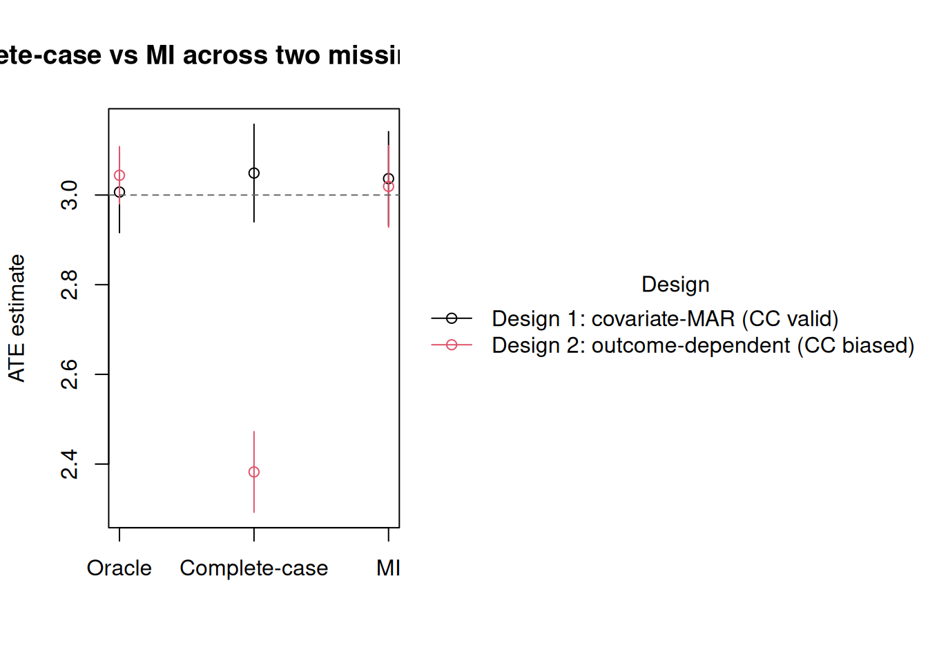
Design 2 is where MI earns its keep: complete-case misses the truth by a wide margin, MI lands on it. Design 1 is the honest counterweight — when complete-case is valid, MI buys nothing and costs a little precision.
causat_mice() is estimator-agnostic — swap estimator = "ipw", "aipw", "matching", or "snm", change the outcome family, the contrast scale, add by = stratification, or go longitudinal with id =/time =, and the same pooling applies. For "ipw" and "matching" MI is not just better but necessary: those engines abort on a missing confounder, so the only alternatives are manual listwise deletion or imputation. MAR treatment is handled the same way: impute A (as a factor, so mice uses logistic regression) and pass the mids object on.
The default pool_method = "rubin" is exactly valid when the imputation and analysis models are congenial. Causal estimands are often uncongenial with the mice model, and under uncongeniality Rubin’s variance can be biased in either direction (Meng 1994; Bartlett and Hughes 2020) — not reliably conservative. pool_method = "boot_mi" (Hippel 2020) replaces Rubin’s variance decomposition with a bootstrap-then-impute resampling variance:
boot_res <- causat_mice(
  imp,
  outcome = "Y",
  treatment = "A",
  confounders = ~L,
  interventions = list(a1 = static(1), a0 = static(0)),
  estimator = "gcomp",
  type = "difference",
  pool_method = "boot_mi",
  B = 50, # raise to ~200-1000 in practice; small here for a fast vignette
  M = 2,
  seed = 1
)
#> Warning: `model_fn` not specified; defaulting to `stats::glm`.
#> ℹ Set `model_fn` explicitly (e.g. `model_fn = stats::glm` or `model_fn = mgcv::gam`).
#> `model_fn` not specified; defaulting to `stats::glm`.
#> ℹ Set `model_fn` explicitly (e.g. `model_fn = stats::glm` or `model_fn = mgcv::gam`).
#> `model_fn` not specified; defaulting to `stats::glm`.
#> ℹ Set `model_fn` explicitly (e.g. `model_fn = stats::glm` or `model_fn = mgcv::gam`).
#> `model_fn` not specified; defaulting to `stats::glm`.
#> ℹ Set `model_fn` explicitly (e.g. `model_fn = stats::glm` or `model_fn = mgcv::gam`).
#> `model_fn` not specified; defaulting to `stats::glm`.
#> ℹ Set `model_fn` explicitly (e.g. `model_fn = stats::glm` or `model_fn = mgcv::gam`).
#> `model_fn` not specified; defaulting to `stats::glm`.
#> ℹ Set `model_fn` explicitly (e.g. `model_fn = stats::glm` or `model_fn = mgcv::gam`).
#> `model_fn` not specified; defaulting to `stats::glm`.
#> ℹ Set `model_fn` explicitly (e.g. `model_fn = stats::glm` or `model_fn = mgcv::gam`).
#> `model_fn` not specified; defaulting to `stats::glm`.
#> ℹ Set `model_fn` explicitly (e.g. `model_fn = stats::glm` or `model_fn = mgcv::gam`).
#> `model_fn` not specified; defaulting to `stats::glm`.
#> ℹ Set `model_fn` explicitly (e.g. `model_fn = stats::glm` or `model_fn = mgcv::gam`).
#> `model_fn` not specified; defaulting to `stats::glm`.
#> ℹ Set `model_fn` explicitly (e.g. `model_fn = stats::glm` or `model_fn = mgcv::gam`).
#> `model_fn` not specified; defaulting to `stats::glm`.
#> ℹ Set `model_fn` explicitly (e.g. `model_fn = stats::glm` or `model_fn = mgcv::gam`).
#> `model_fn` not specified; defaulting to `stats::glm`.
#> ℹ Set `model_fn` explicitly (e.g. `model_fn = stats::glm` or `model_fn = mgcv::gam`).
#> `model_fn` not specified; defaulting to `stats::glm`.
#> ℹ Set `model_fn` explicitly (e.g. `model_fn = stats::glm` or `model_fn = mgcv::gam`).
#> `model_fn` not specified; defaulting to `stats::glm`.
#> ℹ Set `model_fn` explicitly (e.g. `model_fn = stats::glm` or `model_fn = mgcv::gam`).
#> `model_fn` not specified; defaulting to `stats::glm`.
#> ℹ Set `model_fn` explicitly (e.g. `model_fn = stats::glm` or `model_fn = mgcv::gam`).
#> `model_fn` not specified; defaulting to `stats::glm`.
#> ℹ Set `model_fn` explicitly (e.g. `model_fn = stats::glm` or `model_fn = mgcv::gam`).
#> `model_fn` not specified; defaulting to `stats::glm`.
#> ℹ Set `model_fn` explicitly (e.g. `model_fn = stats::glm` or `model_fn = mgcv::gam`).
#> `model_fn` not specified; defaulting to `stats::glm`.
#> ℹ Set `model_fn` explicitly (e.g. `model_fn = stats::glm` or `model_fn = mgcv::gam`).
#> `model_fn` not specified; defaulting to `stats::glm`.
#> ℹ Set `model_fn` explicitly (e.g. `model_fn = stats::glm` or `model_fn = mgcv::gam`).
#> `model_fn` not specified; defaulting to `stats::glm`.
#> ℹ Set `model_fn` explicitly (e.g. `model_fn = stats::glm` or `model_fn = mgcv::gam`).
#> `model_fn` not specified; defaulting to `stats::glm`.
#> ℹ Set `model_fn` explicitly (e.g. `model_fn = stats::glm` or `model_fn = mgcv::gam`).
#> `model_fn` not specified; defaulting to `stats::glm`.
#> ℹ Set `model_fn` explicitly (e.g. `model_fn = stats::glm` or `model_fn = mgcv::gam`).
#> `model_fn` not specified; defaulting to `stats::glm`.
#> ℹ Set `model_fn` explicitly (e.g. `model_fn = stats::glm` or `model_fn = mgcv::gam`).
#> `model_fn` not specified; defaulting to `stats::glm`.
#> ℹ Set `model_fn` explicitly (e.g. `model_fn = stats::glm` or `model_fn = mgcv::gam`).
#> `model_fn` not specified; defaulting to `stats::glm`.
#> ℹ Set `model_fn` explicitly (e.g. `model_fn = stats::glm` or `model_fn = mgcv::gam`).
#> `model_fn` not specified; defaulting to `stats::glm`.
#> ℹ Set `model_fn` explicitly (e.g. `model_fn = stats::glm` or `model_fn = mgcv::gam`).
#> `model_fn` not specified; defaulting to `stats::glm`.
#> ℹ Set `model_fn` explicitly (e.g. `model_fn = stats::glm` or `model_fn = mgcv::gam`).
#> `model_fn` not specified; defaulting to `stats::glm`.
#> ℹ Set `model_fn` explicitly (e.g. `model_fn = stats::glm` or `model_fn = mgcv::gam`).
#> `model_fn` not specified; defaulting to `stats::glm`.
#> ℹ Set `model_fn` explicitly (e.g. `model_fn = stats::glm` or `model_fn = mgcv::gam`).
#> `model_fn` not specified; defaulting to `stats::glm`.
#> ℹ Set `model_fn` explicitly (e.g. `model_fn = stats::glm` or `model_fn = mgcv::gam`).
#> `model_fn` not specified; defaulting to `stats::glm`.
#> ℹ Set `model_fn` explicitly (e.g. `model_fn = stats::glm` or `model_fn = mgcv::gam`).
#> `model_fn` not specified; defaulting to `stats::glm`.
#> ℹ Set `model_fn` explicitly (e.g. `model_fn = stats::glm` or `model_fn = mgcv::gam`).
#> `model_fn` not specified; defaulting to `stats::glm`.
#> ℹ Set `model_fn` explicitly (e.g. `model_fn = stats::glm` or `model_fn = mgcv::gam`).
#> `model_fn` not specified; defaulting to `stats::glm`.
#> ℹ Set `model_fn` explicitly (e.g. `model_fn = stats::glm` or `model_fn = mgcv::gam`).
#> `model_fn` not specified; defaulting to `stats::glm`.
#> ℹ Set `model_fn` explicitly (e.g. `model_fn = stats::glm` or `model_fn = mgcv::gam`).
#> `model_fn` not specified; defaulting to `stats::glm`.
#> ℹ Set `model_fn` explicitly (e.g. `model_fn = stats::glm` or `model_fn = mgcv::gam`).
#> `model_fn` not specified; defaulting to `stats::glm`.
#> ℹ Set `model_fn` explicitly (e.g. `model_fn = stats::glm` or `model_fn = mgcv::gam`).
#> `model_fn` not specified; defaulting to `stats::glm`.
#> ℹ Set `model_fn` explicitly (e.g. `model_fn = stats::glm` or `model_fn = mgcv::gam`).
#> `model_fn` not specified; defaulting to `stats::glm`.
#> ℹ Set `model_fn` explicitly (e.g. `model_fn = stats::glm` or `model_fn = mgcv::gam`).
#> `model_fn` not specified; defaulting to `stats::glm`.
#> ℹ Set `model_fn` explicitly (e.g. `model_fn = stats::glm` or `model_fn = mgcv::gam`).
#> `model_fn` not specified; defaulting to `stats::glm`.
#> ℹ Set `model_fn` explicitly (e.g. `model_fn = stats::glm` or `model_fn = mgcv::gam`).
#> `model_fn` not specified; defaulting to `stats::glm`.
#> ℹ Set `model_fn` explicitly (e.g. `model_fn = stats::glm` or `model_fn = mgcv::gam`).
#> `model_fn` not specified; defaulting to `stats::glm`.
#> ℹ Set `model_fn` explicitly (e.g. `model_fn = stats::glm` or `model_fn = mgcv::gam`).
#> `model_fn` not specified; defaulting to `stats::glm`.
#> ℹ Set `model_fn` explicitly (e.g. `model_fn = stats::glm` or `model_fn = mgcv::gam`).
#> `model_fn` not specified; defaulting to `stats::glm`.
#> ℹ Set `model_fn` explicitly (e.g. `model_fn = stats::glm` or `model_fn = mgcv::gam`).
#> `model_fn` not specified; defaulting to `stats::glm`.
#> ℹ Set `model_fn` explicitly (e.g. `model_fn = stats::glm` or `model_fn = mgcv::gam`).
#> `model_fn` not specified; defaulting to `stats::glm`.
#> ℹ Set `model_fn` explicitly (e.g. `model_fn = stats::glm` or `model_fn = mgcv::gam`).
#> `model_fn` not specified; defaulting to `stats::glm`.
#> ℹ Set `model_fn` explicitly (e.g. `model_fn = stats::glm` or `model_fn = mgcv::gam`).
#> `model_fn` not specified; defaulting to `stats::glm`.
#> ℹ Set `model_fn` explicitly (e.g. `model_fn = stats::glm` or `model_fn = mgcv::gam`).
#> `model_fn` not specified; defaulting to `stats::glm`.
#> ℹ Set `model_fn` explicitly (e.g. `model_fn = stats::glm` or `model_fn = mgcv::gam`).
#> `model_fn` not specified; defaulting to `stats::glm`.
#> ℹ Set `model_fn` explicitly (e.g. `model_fn = stats::glm` or `model_fn = mgcv::gam`).
#> `model_fn` not specified; defaulting to `stats::glm`.
#> ℹ Set `model_fn` explicitly (e.g. `model_fn = stats::glm` or `model_fn = mgcv::gam`).
#> `model_fn` not specified; defaulting to `stats::glm`.
#> ℹ Set `model_fn` explicitly (e.g. `model_fn = stats::glm` or `model_fn = mgcv::gam`).
#> `model_fn` not specified; defaulting to `stats::glm`.
#> ℹ Set `model_fn` explicitly (e.g. `model_fn = stats::glm` or `model_fn = mgcv::gam`).
#> `model_fn` not specified; defaulting to `stats::glm`.
#> ℹ Set `model_fn` explicitly (e.g. `model_fn = stats::glm` or `model_fn = mgcv::gam`).
#> `model_fn` not specified; defaulting to `stats::glm`.
#> ℹ Set `model_fn` explicitly (e.g. `model_fn = stats::glm` or `model_fn = mgcv::gam`).
#> `model_fn` not specified; defaulting to `stats::glm`.
#> ℹ Set `model_fn` explicitly (e.g. `model_fn = stats::glm` or `model_fn = mgcv::gam`).
#> `model_fn` not specified; defaulting to `stats::glm`.
#> ℹ Set `model_fn` explicitly (e.g. `model_fn = stats::glm` or `model_fn = mgcv::gam`).
#> `model_fn` not specified; defaulting to `stats::glm`.
#> ℹ Set `model_fn` explicitly (e.g. `model_fn = stats::glm` or `model_fn = mgcv::gam`).
#> `model_fn` not specified; defaulting to `stats::glm`.
#> ℹ Set `model_fn` explicitly (e.g. `model_fn = stats::glm` or `model_fn = mgcv::gam`).
#> `model_fn` not specified; defaulting to `stats::glm`.
#> ℹ Set `model_fn` explicitly (e.g. `model_fn = stats::glm` or `model_fn = mgcv::gam`).
#> `model_fn` not specified; defaulting to `stats::glm`.
#> ℹ Set `model_fn` explicitly (e.g. `model_fn = stats::glm` or `model_fn = mgcv::gam`).
#> `model_fn` not specified; defaulting to `stats::glm`.
#> ℹ Set `model_fn` explicitly (e.g. `model_fn = stats::glm` or `model_fn = mgcv::gam`).
#> `model_fn` not specified; defaulting to `stats::glm`.
#> ℹ Set `model_fn` explicitly (e.g. `model_fn = stats::glm` or `model_fn = mgcv::gam`).
#> `model_fn` not specified; defaulting to `stats::glm`.
#> ℹ Set `model_fn` explicitly (e.g. `model_fn = stats::glm` or `model_fn = mgcv::gam`).
#> `model_fn` not specified; defaulting to `stats::glm`.
#> ℹ Set `model_fn` explicitly (e.g. `model_fn = stats::glm` or `model_fn = mgcv::gam`).
#> `model_fn` not specified; defaulting to `stats::glm`.
#> ℹ Set `model_fn` explicitly (e.g. `model_fn = stats::glm` or `model_fn = mgcv::gam`).
#> `model_fn` not specified; defaulting to `stats::glm`.
#> ℹ Set `model_fn` explicitly (e.g. `model_fn = stats::glm` or `model_fn = mgcv::gam`).
#> `model_fn` not specified; defaulting to `stats::glm`.
#> ℹ Set `model_fn` explicitly (e.g. `model_fn = stats::glm` or `model_fn = mgcv::gam`).
#> `model_fn` not specified; defaulting to `stats::glm`.
#> ℹ Set `model_fn` explicitly (e.g. `model_fn = stats::glm` or `model_fn = mgcv::gam`).
#> `model_fn` not specified; defaulting to `stats::glm`.
#> ℹ Set `model_fn` explicitly (e.g. `model_fn = stats::glm` or `model_fn = mgcv::gam`).
#> `model_fn` not specified; defaulting to `stats::glm`.
#> ℹ Set `model_fn` explicitly (e.g. `model_fn = stats::glm` or `model_fn = mgcv::gam`).
#> `model_fn` not specified; defaulting to `stats::glm`.
#> ℹ Set `model_fn` explicitly (e.g. `model_fn = stats::glm` or `model_fn = mgcv::gam`).
#> `model_fn` not specified; defaulting to `stats::glm`.
#> ℹ Set `model_fn` explicitly (e.g. `model_fn = stats::glm` or `model_fn = mgcv::gam`).
#> `model_fn` not specified; defaulting to `stats::glm`.
#> ℹ Set `model_fn` explicitly (e.g. `model_fn = stats::glm` or `model_fn = mgcv::gam`).
#> `model_fn` not specified; defaulting to `stats::glm`.
#> ℹ Set `model_fn` explicitly (e.g. `model_fn = stats::glm` or `model_fn = mgcv::gam`).
#> `model_fn` not specified; defaulting to `stats::glm`.
#> ℹ Set `model_fn` explicitly (e.g. `model_fn = stats::glm` or `model_fn = mgcv::gam`).
#> `model_fn` not specified; defaulting to `stats::glm`.
#> ℹ Set `model_fn` explicitly (e.g. `model_fn = stats::glm` or `model_fn = mgcv::gam`).
#> `model_fn` not specified; defaulting to `stats::glm`.
#> ℹ Set `model_fn` explicitly (e.g. `model_fn = stats::glm` or `model_fn = mgcv::gam`).
#> `model_fn` not specified; defaulting to `stats::glm`.
#> ℹ Set `model_fn` explicitly (e.g. `model_fn = stats::glm` or `model_fn = mgcv::gam`).
#> `model_fn` not specified; defaulting to `stats::glm`.
#> ℹ Set `model_fn` explicitly (e.g. `model_fn = stats::glm` or `model_fn = mgcv::gam`).
#> `model_fn` not specified; defaulting to `stats::glm`.
#> ℹ Set `model_fn` explicitly (e.g. `model_fn = stats::glm` or `model_fn = mgcv::gam`).
#> `model_fn` not specified; defaulting to `stats::glm`.
#> ℹ Set `model_fn` explicitly (e.g. `model_fn = stats::glm` or `model_fn = mgcv::gam`).
#> `model_fn` not specified; defaulting to `stats::glm`.
#> ℹ Set `model_fn` explicitly (e.g. `model_fn = stats::glm` or `model_fn = mgcv::gam`).
#> `model_fn` not specified; defaulting to `stats::glm`.
#> ℹ Set `model_fn` explicitly (e.g. `model_fn = stats::glm` or `model_fn = mgcv::gam`).
#> `model_fn` not specified; defaulting to `stats::glm`.
#> ℹ Set `model_fn` explicitly (e.g. `model_fn = stats::glm` or `model_fn = mgcv::gam`).
#> `model_fn` not specified; defaulting to `stats::glm`.
#> ℹ Set `model_fn` explicitly (e.g. `model_fn = stats::glm` or `model_fn = mgcv::gam`).
#> `model_fn` not specified; defaulting to `stats::glm`.
#> ℹ Set `model_fn` explicitly (e.g. `model_fn = stats::glm` or `model_fn = mgcv::gam`).
#> `model_fn` not specified; defaulting to `stats::glm`.
#> ℹ Set `model_fn` explicitly (e.g. `model_fn = stats::glm` or `model_fn = mgcv::gam`).
#> `model_fn` not specified; defaulting to `stats::glm`.
#> ℹ Set `model_fn` explicitly (e.g. `model_fn = stats::glm` or `model_fn = mgcv::gam`).
#> `model_fn` not specified; defaulting to `stats::glm`.
#> ℹ Set `model_fn` explicitly (e.g. `model_fn = stats::glm` or `model_fn = mgcv::gam`).
#> `model_fn` not specified; defaulting to `stats::glm`.
#> ℹ Set `model_fn` explicitly (e.g. `model_fn = stats::glm` or `model_fn = mgcv::gam`).
#> `model_fn` not specified; defaulting to `stats::glm`.
#> ℹ Set `model_fn` explicitly (e.g. `model_fn = stats::glm` or `model_fn = mgcv::gam`).
#> `model_fn` not specified; defaulting to `stats::glm`.
#> ℹ Set `model_fn` explicitly (e.g. `model_fn = stats::glm` or `model_fn = mgcv::gam`).
#> `model_fn` not specified; defaulting to `stats::glm`.
#> ℹ Set `model_fn` explicitly (e.g. `model_fn = stats::glm` or `model_fn = mgcv::gam`).
#> `model_fn` not specified; defaulting to `stats::glm`.
#> ℹ Set `model_fn` explicitly (e.g. `model_fn = stats::glm` or `model_fn = mgcv::gam`).
#> `model_fn` not specified; defaulting to `stats::glm`.
#> ℹ Set `model_fn` explicitly (e.g. `model_fn = stats::glm` or `model_fn = mgcv::gam`).
#> `model_fn` not specified; defaulting to `stats::glm`.
#> ℹ Set `model_fn` explicitly (e.g. `model_fn = stats::glm` or `model_fn = mgcv::gam`).
#> `model_fn` not specified; defaulting to `stats::glm`.
#> ℹ Set `model_fn` explicitly (e.g. `model_fn = stats::glm` or `model_fn = mgcv::gam`).
#> `model_fn` not specified; defaulting to `stats::glm`.
#> ℹ Set `model_fn` explicitly (e.g. `model_fn = stats::glm` or `model_fn = mgcv::gam`).
boot_res
Estimator: gcomp · Estimand: ATE · Contrast: difference · CI method: boot_mi · N: 2000
| intervention | estimate | se | ci_lower | ci_upper |
|---|---|---|---|---|
| a1 | 5.04 | 0.049 | 4.942 | 5.137 |
| a0 | 2.001 | 0.051 | 1.898 | 2.104 |
| comparison | estimate | se | ci_lower | ci_upper |
|---|---|---|---|---|
| a0 vs a1 | -3.039 | 0.045 | -3.13 | -2.948 |
Both pooling rules are only as good as the consistency of the underlying estimator — the next note explains why that puts the outcome in the imputation model.
A bootstrap (and Rubin’s rules) corrects the variance, not bias in the point estimate. Both pooling rules attain approximately nominal coverage only when the causal estimator stays consistent (Bartlett and Hughes 2020). The single most important way to keep it consistent is to include the outcome Y as a predictor in the imputation model (Buuren 2018, ch. 6): omitting it produces biased imputed covariates, which biases the causal estimate — and no pooling rule can repair that.
Design 2 makes the stakes concrete. Re-impute it with Y excluded from the predictor matrix — exactly the misspecification the missingness mechanism punishes — and the MI estimate is biased further from the truth than even complete-case. causat_mice() flags it: it warns when an analysis variable is absent from, or unused by, the imputation model.
pred <- mice::make.predictorMatrix(df2)
pred[, "Y"] <- 0 # deliberately drop Y from the predictor matrix
imp_noY <- mice(df2, predictorMatrix = pred, m = 20, printFlag = FALSE)

# The warning fires: Y is present in the data but never used to impute L.
mi_noY <- causat_mice(
  imp_noY,
  outcome = "Y",
  treatment = "A",
  confounders = ~L,
  interventions = list(a1 = static(1), a0 = static(0)),
  estimator = "gcomp"
)
#> Warning: Some analysis variables are not used by the imputation model.
#> ✖ Absent or never used as a predictor: `Y`.
#> ℹ Include all analysis variables (outcome, treatment, confounders, effect modifiers) as predictors in `mice::mice()` to reduce bias and uncongeniality.
#> Warning: `model_fn` not specified; defaulting to `stats::glm`.
#> ℹ Set `model_fn` explicitly (e.g. `model_fn = stats::glm` or `model_fn = mgcv::gam`).
#> `model_fn` not specified; defaulting to `stats::glm`.
#> ℹ Set `model_fn` explicitly (e.g. `model_fn = stats::glm` or `model_fn = mgcv::gam`).
#> `model_fn` not specified; defaulting to `stats::glm`.
#> ℹ Set `model_fn` explicitly (e.g. `model_fn = stats::glm` or `model_fn = mgcv::gam`).
#> `model_fn` not specified; defaulting to `stats::glm`.
#> ℹ Set `model_fn` explicitly (e.g. `model_fn = stats::glm` or `model_fn = mgcv::gam`).
#> `model_fn` not specified; defaulting to `stats::glm`.
#> ℹ Set `model_fn` explicitly (e.g. `model_fn = stats::glm` or `model_fn = mgcv::gam`).
#> `model_fn` not specified; defaulting to `stats::glm`.
#> ℹ Set `model_fn` explicitly (e.g. `model_fn = stats::glm` or `model_fn = mgcv::gam`).
#> `model_fn` not specified; defaulting to `stats::glm`.
#> ℹ Set `model_fn` explicitly (e.g. `model_fn = stats::glm` or `model_fn = mgcv::gam`).
#> `model_fn` not specified; defaulting to `stats::glm`.
#> ℹ Set `model_fn` explicitly (e.g. `model_fn = stats::glm` or `model_fn = mgcv::gam`).
#> `model_fn` not specified; defaulting to `stats::glm`.
#> ℹ Set `model_fn` explicitly (e.g. `model_fn = stats::glm` or `model_fn = mgcv::gam`).
#> `model_fn` not specified; defaulting to `stats::glm`.
#> ℹ Set `model_fn` explicitly (e.g. `model_fn = stats::glm` or `model_fn = mgcv::gam`).
#> `model_fn` not specified; defaulting to `stats::glm`.
#> ℹ Set `model_fn` explicitly (e.g. `model_fn = stats::glm` or `model_fn = mgcv::gam`).
#> `model_fn` not specified; defaulting to `stats::glm`.
#> ℹ Set `model_fn` explicitly (e.g. `model_fn = stats::glm` or `model_fn = mgcv::gam`).
#> `model_fn` not specified; defaulting to `stats::glm`.
#> ℹ Set `model_fn` explicitly (e.g. `model_fn = stats::glm` or `model_fn = mgcv::gam`).
#> `model_fn` not specified; defaulting to `stats::glm`.
#> ℹ Set `model_fn` explicitly (e.g. `model_fn = stats::glm` or `model_fn = mgcv::gam`).
#> `model_fn` not specified; defaulting to `stats::glm`.
#> ℹ Set `model_fn` explicitly (e.g. `model_fn = stats::glm` or `model_fn = mgcv::gam`).
#> `model_fn` not specified; defaulting to `stats::glm`.
#> ℹ Set `model_fn` explicitly (e.g. `model_fn = stats::glm` or `model_fn = mgcv::gam`).
#> `model_fn` not specified; defaulting to `stats::glm`.
#> ℹ Set `model_fn` explicitly (e.g. `model_fn = stats::glm` or `model_fn = mgcv::gam`).
#> `model_fn` not specified; defaulting to `stats::glm`.
#> ℹ Set `model_fn` explicitly (e.g. `model_fn = stats::glm` or `model_fn = mgcv::gam`).
#> `model_fn` not specified; defaulting to `stats::glm`.
#> ℹ Set `model_fn` explicitly (e.g. `model_fn = stats::glm` or `model_fn = mgcv::gam`).
#> `model_fn` not specified; defaulting to `stats::glm`.
#> ℹ Set `model_fn` explicitly (e.g. `model_fn = stats::glm` or `model_fn = mgcv::gam`).| Method | Estimate |
|---|---|
| Complete-case | 2.382 |
| MI (Y included) | 3.019 |
| MI (Y excluded) | 3.919 |
So MI is not automatically safe: done well (with Y) it recovers the truth that complete-case missed; done badly (without Y) it can be worse than complete-case. The imputation model matters.
Do not impute Y itself: missing outcomes belong to inverse-probability-of- censoring weighting (ipcw = TRUE, shown below) or complete-case analysis, not MI. Including Y as a predictor (good) is the opposite of imputing Y (wrong tool).
causatr gracefully handles the case where both Y and L have missing values (possibly on different rows):
df_both <- df
df_both$Y[sample(n, round(0.10 * n))] <- NA
df_both$L1[sample(n, round(0.10 * n))] <- NA

fit_both <- causat(
  df_both,
  outcome = "Y",
  treatment = "A",
  confounders = ~ L1 + L2,
  model_fn = stats::glm
)

res_both <- contrast(
  fit_both,
  interventions = list(a1 = static(1), a0 = static(0)),
  reference = "a0",
  type = "difference",
  ci_method = "sandwich"
)
#> 200 row(s) with NA predictions excluded from the target population.
res_both
Estimator: gcomp · Estimand: ATE · Contrast: difference · CI method: sandwich · N: 1800
| intervention | estimate | se | ci_lower | ci_upper |
|---|---|---|---|---|
| a1 | 4.986 | 0.054 | 4.881 | 5.091 |
| a0 | 1.993 | 0.054 | 1.886 | 2.099 |
| comparison | estimate | se | ci_lower | ci_upper |
|---|---|---|---|---|
| a1 vs a0 | 2.993 | 0.051 | 2.892 | 3.094 |
Treatment NAs are not allowed — you cannot define a counterfactual without knowing the observed treatment value. causatr aborts with an informative error:
df_a_miss <- df
df_a_miss$A[1:10] <- NA

causat(
  df_a_miss,
  outcome = "Y",
  treatment = "A",
  confounders = ~ L1 + L2,
  model_fn = stats::glm
)
#> Error in `causat()`:
#> ! Treatment variable 'A' has 10 missing values.
#> ℹ Use `censoring = '...'` for inverse probability of censoring weights.
#> ℹ Or impute upstream with `mice::mice()` and pool with `causat_mice()` (multiple imputation for MAR treatment).
#> ℹ Or remove incomplete cases before calling `causat()`.
If treatment is MCAR, drop the rows. If MAR, impute A with mice() (store it as a factor so mice uses logistic regression) and pool with causat_mice(), exactly as for a MAR covariate above.
The same principles apply to continuous treatments. Here we show IPW with a shift() intervention under outcome missingness.
Data-generating mechanism. A single confounder \(L\) affects both a continuous treatment \(A\) and a continuous outcome \(Y\). The treatment is Gaussian with its mean depending on \(L\), and the outcome is linear in \(A\) and \(L\).
\[ \begin{aligned} L &\sim \mathcal{N}(0, 1) \\ A &\sim \mathcal{N}(0.5\,L,\; 1) \\ Y &= 1 + 2\,A + L + \varepsilon, \quad \varepsilon \sim \mathcal{N}(0, 1) \end{aligned} \]
Under a unit additive shift intervention \(A^* = A + 1\), every individual’s treatment increases by 1 and the outcome increases by \(2 \times 1 = 2\). The true causal contrast is \(E[Y(A+1)] - E[Y(A)] = 2\).
set.seed(43)
L <- rnorm(n)
A_cont <- rnorm(n, mean = 0.5 * L)
Y_cont <- 1 + 2 * A_cont + L + rnorm(n)
df_cont <- data.frame(Y = Y_cont, A = A_cont, L = L)
df_cont$Y[sample(n, round(0.10 * n))] <- NA

fit_cont_ipw <- causat(
  df_cont,
  outcome = "Y",
  treatment = "A",
  confounders = ~ L,
  estimator = "ipw",
  model_fn = stats::glm,
  propensity_model_fn = stats::glm
)

res_cont_ipw <- contrast(
  fit_cont_ipw,
  interventions = list(up1 = shift(1), observed = NULL),
  reference = "observed",
  type = "difference",
  ci_method = "sandwich"
)
res_cont_ipw
Estimator: ipw · Estimand: ATE · Contrast: difference · CI method: sandwich · N: 2000
| intervention | estimate | se | ci_lower | ci_upper |
|---|---|---|---|---|
| up1 | 3.043 | 0.135 | 2.779 | 3.307 |
| observed | 1.029 | 0.071 | 0.889 | 1.169 |
| comparison | estimate | se | ci_lower | ci_upper |
|---|---|---|---|---|
| up1 vs observed | 2.014 | 0.114 | 1.791 | 2.237 |
Structural truth: E[Y(A+1)] - E[Y(A)] = 2.
G-comp handles missing outcomes for categorical treatments.
Data-generating mechanism. A three-arm categorical treatment \(A \in \{A, B, C\}\) is drawn independently of the confounder \(L\), and the outcome depends on both the treatment arm and \(L\).
\[ \begin{aligned} A &\sim \text{Categorical}(0.3,\; 0.4,\; 0.3) \\ L &\sim \mathcal{N}(0, 1) \\ Y &= 1 + \mathbf{1}(A = B) \cdot 1 + \mathbf{1}(A = C) \cdot 2 + 0.5\,L + \varepsilon, \quad \varepsilon \sim \mathcal{N}(0, 1) \end{aligned} \]
The true contrasts relative to arm A are: \(E[Y^{B}] - E[Y^{A}] = 1\) and \(E[Y^{C}] - E[Y^{A}] = 2\).
set.seed(44)
A_cat <- factor(
  sample(c("A", "B", "C"), n, replace = TRUE, prob = c(0.3, 0.4, 0.3))
)
L <- rnorm(n)
Y_cat <- 1 +
  ifelse(A_cat == "B", 1, ifelse(A_cat == "C", 2, 0)) +
  0.5 * L + rnorm(n)
df_cat <- data.frame(Y = Y_cat, A = A_cat, L = L)
df_cat$Y[sample(n, round(0.10 * n))] <- NA

fit_cat <- causat(
  df_cat,
  outcome = "Y",
  treatment = "A",
  confounders = ~ L,
  model_fn = stats::glm
)

res_cat <- contrast(
  fit_cat,
  interventions = list(
    arm_a = static("A"),
    arm_b = static("B"),
    arm_c = static("C")
  ),
  reference = "arm_a",
  type = "difference",
  ci_method = "sandwich"
)
res_cat
Estimator: gcomp · Estimand: ATE · Contrast: difference · CI method: sandwich · N: 2000
| intervention | estimate | se | ci_lower | ci_upper |
|---|---|---|---|---|
| arm_a | 0.999 | 0.046 | 0.909 | 1.089 |
| arm_b | 1.976 | 0.039 | 1.899 | 2.054 |
| arm_c | 3.005 | 0.042 | 2.923 | 3.088 |
| comparison | estimate | se | ci_lower | ci_upper |
|---|---|---|---|---|
| arm_b vs arm_a | 0.977 | 0.059 | 0.863 | 1.092 |
| arm_c vs arm_a | 2.006 | 0.06 | 1.888 | 2.125 |
ICE g-computation handles missing final-period outcomes. The backward recursion excludes NA rows when fitting each sequential outcome model.
Data-generating mechanism. A two-period panel (\(K = 2\)) with \(n = 500\) individuals. Each individual has a baseline confounder \(L_0\), a time-varying confounder \(L_k\), and a binary treatment \(A_k\) at each period. The outcome \(Y\) is observed only at the final period and depends on the cumulative treatment received across both periods.
\[ \begin{aligned} L_0 &\sim \mathcal{N}(0, 1) \\ L_k &= L_0 + \eta_k, \quad \eta_k \sim \mathcal{N}(0, 0.25) \\ A_k &\sim \text{Bernoulli}\bigl(\text{logit}^{-1}(0.3\,L_k)\bigr), \quad k = 1, 2 \\ Y &= 2 + 1.5\,(A_1 + A_2) + 0.5\,L_0 + \varepsilon, \quad \varepsilon \sim \mathcal{N}(0, 1) \end{aligned} \]
Under the “always treat” regime (\(A_1 = A_2 = 1\)) vs “never treat” (\(A_1 = A_2 = 0\)), the true ATE is \(1.5 \times 2 = 3\).
set.seed(45)
n_id <- 500
ids <- rep(seq_len(n_id), each = 2)
times <- rep(1:2, n_id)
L0 <- rep(rnorm(n_id), each = 2)
L_tv <- L0 + rnorm(n_id * 2, 0, 0.5)
A_tv <- rbinom(n_id * 2, 1, plogis(0.3 * L_tv))

Y_long <- NA_real_
for (i in seq_len(n_id)) {
  rows <- which(ids == i)
  Y_long[rows[2]] <- 2 + 1.5 * sum(A_tv[rows]) + 0.5 * L0[rows[1]] + rnorm(1)
}

long_df <- data.frame(
  id = ids, time = times, Y = Y_long, A = A_tv, L0 = L0, L = L_tv
)
long_df$Y[sample(which(!is.na(long_df$Y)), round(0.10 * n_id))] <- NA

fit_ice_miss <- causat(
  long_df,
  outcome = "Y",
  treatment = "A",
  confounders = ~ L0,
  confounders_tv = ~ L,
  id = "id",
  time = "time",
  model_fn = stats::glm
)

res_ice_miss <- contrast(
  fit_ice_miss,
  interventions = list(always = static(1), never = static(0)),
  reference = "never",
  type = "difference",
  ci_method = "sandwich"
)
res_ice_miss
Estimator: gcomp · Estimand: ATE · Contrast: difference · CI method: sandwich · N: 500
| intervention | estimate | se | ci_lower | ci_upper |
|---|---|---|---|---|
| always | 4.991 | 0.085 | 4.825 | 5.158 |
| never | 1.905 | 0.089 | 1.731 | 2.079 |
| comparison | estimate | se | ci_lower | ci_upper |
|---|---|---|---|---|
| always vs never | 3.086 | 0.14 | 2.812 | 3.361 |
Structural truth: ATE = 1.5 * 2 = 3 (two periods of binary treatment).
Bootstrap inference correctly handles missing data — each replicate resamples individuals (with replacement) and refits the full pipeline:
res_boot_miss <- contrast(
  fit_y,
  interventions = list(a1 = static(1), a0 = static(0)),
  reference = "a0",
  type = "difference",
  ci_method = "bootstrap",
  n_boot = 50L
)
res_boot_miss
Estimator: gcomp · Estimand: ATE · Contrast: difference · CI method: bootstrap · N: 2000
| intervention | estimate | se | ci_lower | ci_upper |
|---|---|---|---|---|
| a1 | 4.966 | 0.051 | 4.895 | 5.077 |
| a0 | 1.955 | 0.054 | 1.873 | 2.097 |
| comparison | estimate | se | ci_lower | ci_upper |
|---|---|---|---|---|
| a1 vs a0 | 3.011 | 0.04 | 2.928 | 3.075 |
boot_comp <- data.frame(
  Inference = c("Sandwich", "Bootstrap"),
  Estimate = c(
    res_y$contrasts$estimate[1], res_boot_miss$contrasts$estimate[1]
  ),
  SE = c(res_y$contrasts$se[1], res_boot_miss$contrasts$se[1]),
  CI_lower = c(
    res_y$contrasts$ci_lower[1], res_boot_miss$contrasts$ci_lower[1]
  ),
  CI_upper = c(
    res_y$contrasts$ci_upper[1], res_boot_miss$contrasts$ci_upper[1]
  )
)
tt(boot_comp, digits = 3)| Inference | Estimate | SE | CI_lower | CI_upper |
|---|---|---|---|---|
| Sandwich | 3.01 | 0.0492 | 2.91 | 3.11 |
| Bootstrap | 3.01 | 0.0402 | 2.93 | 3.07 |
causatr offers two ways to handle outcome censoring via the censoring = argument:
Row filter (censoring = "C", ipcw = FALSE — the default): censored rows are dropped before model fitting. No censoring model is fit. Under g-computation with a correctly specified outcome model this is sufficient for MCAR and MAR censoring (the outcome model adjusts for censoring predictors). Under IPW this is biased for MAR because the treatment model cannot correct for differential censoring.
Built-in IPCW (censoring = "C", ipcw = TRUE): causatr fits an internal censoring model \(P(C = 0 \mid A, L)\) and computes stabilized IPCW weights. These weights are composed multiplicatively with any external weights =. For g-comp this provides doubly-robust protection (correct if either the outcome model or the censoring model is well-specified). For IPW it is essential under MAR. The sandwich SE fully accounts for censoring-model estimation uncertainty (Channel 2 correction).
Custom censoring model. By default the censoring model uses stats::glm. Pass censoring_model_fn = mgcv::gam (or any function with the standard (formula, data, family, weights, ...) signature) to use a more flexible model for the censoring mechanism. Use confounders_censoring to specify a different covariate set for the censoring model than for the outcome or treatment models (e.g. when censoring depends on a different subset of covariates).
ipcw = TRUE)When outcomes are missing at random (MAR) conditional on treatment and covariates, causatr can fit a censoring model \(P(C = 0 \mid A, L)\) internally and compute stabilized IPCW weights. This requires a binary censoring indicator column (1 = censored, 0 = observed) and ipcw = TRUE.
Censoring mechanism. Starting from the baseline DGM above (ATE \(= 3\)), we introduce MAR outcome censoring. The probability of being censored depends on both the treatment \(A\) and confounder \(L_1\):
\[ \begin{aligned} C_i &\sim \text{Bernoulli}\bigl(\text{logit}^{-1}(-2 + 0.5\,A_i + 0.3\,L_{1,i})\bigr) \\ Y_i^{\text{obs}} &= \begin{cases} Y_i & \text{if } C_i = 0 \\ \text{NA} & \text{if } C_i = 1 \end{cases} \end{aligned} \]
The intercept of \(-2\) keeps the censoring rate moderate. Because censoring depends on \(A\) and \(L_1\), a complete-case analysis is biased; IPCW weights restore consistency. The true ATE remains 3.
df_mar <- df
cens_prob <- plogis(-2 + 0.5 * df_mar$A + 0.3 * df_mar$L1)
C <- as.integer(runif(n) < cens_prob)
df_mar$C <- C
df_mar$Y[C == 1L] <- NAfit_ipcw <- causat(
df_mar,
outcome = "Y",
treatment = "A",
confounders = ~ L1 + L2,
censoring = "C",
ipcw = TRUE,
model_fn = stats::glm
)
res_ipcw <- contrast(
fit_ipcw,
interventions = list(a1 = static(1), a0 = static(0)),
reference = "a0",
type = "difference",
ci_method = "sandwich"
)
res_ipcwEstimator: gcomp · Estimand: ATE · Contrast: difference · CI method: sandwich · N: 2000
| intervention | estimate | se | ci_lower | ci_upper |
|---|---|---|---|---|
| a1 | 4.967 | 0.052 | 4.865 | 5.068 |
| a0 | 1.978 | 0.052 | 1.876 | 2.08 |
| comparison | estimate | se | ci_lower | ci_upper |
|---|---|---|---|---|
| a1 vs a0 | 2.988 | 0.05 | 2.89 | 3.086 |
For IPW, IPCW is essential under MAR censoring — without it, the density-ratio weights cannot correct for the selection bias introduced by differential censoring.
fit_ipcw_ipw <- causat(
  df_mar,
  outcome = "Y",
  treatment = "A",
  confounders = ~ L1 + L2,
  estimator = "ipw",
  censoring = "C",
  ipcw = TRUE,
  model_fn = stats::glm,
  propensity_model_fn = stats::glm
)

res_ipcw_ipw <- contrast(
  fit_ipcw_ipw,
  interventions = list(a1 = static(1), a0 = static(0)),
  reference = "a0",
  type = "difference",
  ci_method = "sandwich"
)
res_ipcw_ipw
Estimator: ipw · Estimand: ATE · Contrast: difference · CI method: sandwich · N: 2000
| intervention | estimate | se | ci_lower | ci_upper |
|---|---|---|---|---|
| a1 | 4.974 | 0.05 | 4.876 | 5.073 |
| a0 | 1.989 | 0.051 | 1.89 | 2.089 |
| comparison | estimate | se | ci_lower | ci_upper |
|---|---|---|---|---|
| a1 vs a0 | 2.985 | 0.051 | 2.886 | 3.084 |
fit_naive <- causat(
  df_mar,
  outcome = "Y",
  treatment = "A",
  confounders = ~ L1 + L2,
  censoring = "C",
  model_fn = stats::glm
)
res_naive <- contrast(
  fit_naive,
  interventions = list(a1 = static(1), a0 = static(0)),
  reference = "a0",
  type = "difference",
  ci_method = "sandwich"
)

comp_ipcw <- data.frame(
  Analysis = c("Complete-case (naive)", "G-comp + IPCW", "IPW + IPCW"),
  Estimate = c(
    res_naive$contrasts$estimate[1],
    res_ipcw$contrasts$estimate[1],
    res_ipcw_ipw$contrasts$estimate[1]
  ),
  SE = c(
    res_naive$contrasts$se[1],
    res_ipcw$contrasts$se[1],
    res_ipcw_ipw$contrasts$se[1]
  )
)
tt(comp_ipcw, digits = 3)| Analysis | Estimate | SE |
|---|---|---|
| Complete-case (naive) | 2.99 | 0.0499 |
| G-comp + IPCW | 2.99 | 0.05 |
| IPW + IPCW | 2.99 | 0.0505 |
The IPCW estimates should be closer to the truth (ATE = 3) than naive complete-case analysis:
ipcw_plot_df <- data.frame(
  Method = factor(
    c("Naive (complete-case)", "G-comp + IPCW", "IPW + IPCW"),
    levels = c("Naive (complete-case)", "G-comp + IPCW", "IPW + IPCW")
  ),
  Estimate = c(
    res_naive$contrasts$estimate[1],
    res_ipcw$contrasts$estimate[1],
    res_ipcw_ipw$contrasts$estimate[1]
  ),
  CI_lower = c(
    res_naive$contrasts$ci_lower[1],
    res_ipcw$contrasts$ci_lower[1],
    res_ipcw_ipw$contrasts$ci_lower[1]
  ),
  CI_upper = c(
    res_naive$contrasts$ci_upper[1],
    res_ipcw$contrasts$ci_upper[1],
    res_ipcw_ipw$contrasts$ci_upper[1]
  )
)

tinyplot::tinyplot(
  Estimate ~ Method,
  data = ipcw_plot_df,
  type = "pointrange",
  ymin = ipcw_plot_df$CI_lower,
  ymax = ipcw_plot_df$CI_upper,
  pch = 19,
  ylab = "ATE estimate (95% CI)",
  main = "MAR censoring: naive vs IPCW correction"
)
abline(h = 3, lty = 2, col = "grey40")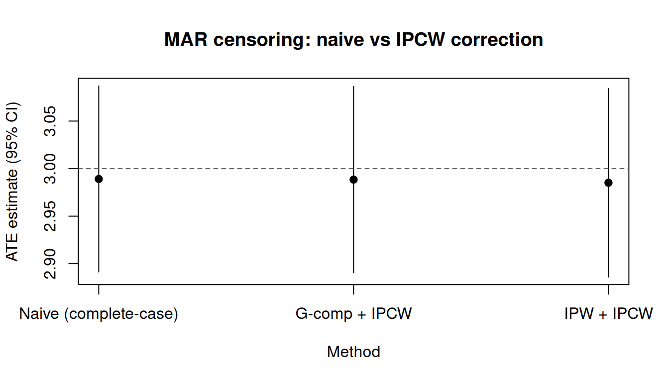
diag_ipcw <- diagnose(fit_ipcw)
#> Note: `s.d.denom` not specified; assuming "pooled".
diag_ipcw
#> <causatr_diag>
#>  Estimator:gcomp
#>  Treatment: binary
#>  Estimand:  ATE
#>
#> Positivity:
#>       statistic     value
#>          <char>     <num>
#>             min 0.2255037
#>             q25 0.4298190
#>          median 0.4861678
#>             q75 0.5451238
#>             max 0.7504067
#>   n_below_lower 0.0000000
#>   n_above_upper 0.0000000
#>    n_violations 0.0000000
#>  pct_violations 0.0000000
#>
#> Covariate balance:
#> Balance Measures
#>       Type Diff.Un     M.Threshold.Un V.Ratio.Un
#> L1 Contin.  0.2690 Not Balanced, >0.1     0.9252
#> L2 Contin.  0.2241 Not Balanced, >0.1     1.0007
#>
#> Balance tally for mean differences
#>                    count
#> Balanced, <0.1         0
#> Not Balanced, >0.1     2
#>
#> Variable with the greatest mean difference
#>  Variable Diff.Un     M.Threshold.Un
#>        L1   0.269 Not Balanced, >0.1
#>
#> Sample sizes
#>     Control Treated
#> All     867     823
#>
#> Censoring:
#>        statistic     value
#>           <char>     <num>
#>          n_total 2000.0000
#>       n_censored  310.0000
#>     pct_censored   15.5000
#>        ipcw_mean    1.0000
#>          ipcw_sd    0.0387
#>         ipcw_min    0.9110
#>         ipcw_max    1.1889
#>         ipcw_ess 1687.4750
#>     p_uncens_min    0.7107
#>     p_uncens_q05    0.7885
#>  p_uncens_median    0.8477
#>     p_uncens_q95    0.8931
#>     p_uncens_max    0.9276
The censoring panel shows IPCW weight summaries and the censoring model’s positivity (predicted \(P(C = 0 \mid A, L)\) quantiles). Watch for extreme weights or near-zero uncensoring probabilities.
weights =For advanced users who want full control over the censoring model, you can compute IPCW weights externally and pass them via weights =:
observed <- !is.na(df$Y) | (df_mar$C == 0L)
cens_model <- glm(observed ~ A + L1 + L2, data = df_mar, family = binomial)
#> Warning: glm.fit: algorithm did not converge
ipcw_manual <- ifelse(observed, 1 / predict(cens_model, type = "response"), 0)

fit_manual_ipcw <- causat(
  df_mar[observed, ],
  outcome = "Y",
  treatment = "A",
  confounders = ~ L1 + L2,
  weights = ipcw_manual[observed],
  model_fn = stats::glm
)

res_manual_ipcw <- contrast(
  fit_manual_ipcw,
  interventions = list(a1 = static(1), a0 = static(0)),
  reference = "a0",
  type = "difference",
  ci_method = "sandwich"
)
res_manual_ipcw
Estimator: gcomp · Estimand: ATE · Contrast: difference · CI method: sandwich · N: 2000
| intervention | estimate | se | ci_lower | ci_upper |
|---|---|---|---|---|
| a1 | 4.967 | 0.052 | 4.866 | 5.069 |
| a0 | 1.978 | 0.052 | 1.877 | 2.08 |
| comparison | estimate | se | ci_lower | ci_upper |
|---|---|---|---|---|
| a1 vs a0 | 2.989 | 0.05 | 2.891 | 3.087 |
Note: with manual IPCW, the sandwich SE does not account for censoring-model estimation uncertainty (the Channel 2 correction). Use ipcw = TRUE for correct standard errors, or ci_method = "bootstrap" with manual weights.
| Variable | Mechanism | Method | Handling | Status |
|---|---|---|---|---|
| Outcome (Y) | MCAR | G-comp | Complete-case model, predict on all rows | Supported |
| Outcome (Y) | MCAR | IPW | Fit treatment model on observed-Y subset | Supported |
| Outcome (Y) | MCAR | Matching | MatchIt excludes NA-Y rows | Supported |
| Outcome (Y) | MAR | Any + ipcw=TRUE | Built-in IPCW via censoring= + ipcw=TRUE | Supported |
| Outcome (Y) | MAR | Any + manual weights | External IPCW weights via weights= | Supported |
| Treatment (A) | NA to causat() | Any | Rejected (abort with error) | Rejected |
| Treatment (A) | MAR | Any | Impute A, then causat_mice() | Supported |
| Covariates (L) | MCAR | G-comp | na.omit drops rows; predict returns NA | Supported |
| Covariates (L) | MAR | Any | Multiple imputation via causat_mice() | Supported |
| Y + L | MCAR | G-comp | Combines both drop rules | Supported |
Missing outcomes (MCAR) are handled automatically by all estimators. The estimate is unbiased; the SE increases proportionally to the information loss.
Missing treatment values cannot be passed to causat() directly. Drop rows (MCAR) or impute with mice() + causat_mice() (MAR).
Missing covariates (MCAR) work out-of-the-box under g-comp via na.omit. For MAR missingness, use multiple imputation via causat_mice() (Rubin’s rules by default, Boot MI when congeniality is in doubt). Always include the outcome as a predictor in the imputation model.
MAR outcome missingness is handled by ipcw = TRUE, which fits a censoring model and computes stabilized IPCW weights automatically. Advanced users can also supply manual IPCW weights via weights =.
Bootstrap handles all missingness patterns correctly by resampling the full pipeline.