Code
library(causatr)
library(tinyplot)

data("nhefs")

nhefs_complete <- nhefs[!is.na(nhefs$wt82_71) & !is.na(nhefs$education), ]causatr separates model fitting (causat()) from causal contrasts (contrast()). The intervention — the hypothetical change in treatment — is specified at contrast time, not fit time. This design lets you fit once and contrast under many different interventions without re-estimating nuisance models.
This vignette tours every intervention constructor, shows which estimators support it, and demonstrates the calling pattern on real and simulated data.
| Constructor | What it does | G-comp | IPW | AIPW | Matching |
|---|---|---|---|---|---|
static(v) |
Set treatment to v for everyone |
All types | Binary, categorical | All types | Binary |
shift(d) |
Add d to observed treatment |
Continuous | Continuous, count (integer d) |
Continuous | — |
scale_by(c) |
Multiply observed treatment by c |
Continuous | Continuous, count (integer-preserving) | Continuous | — |
threshold(lo, hi) |
Clamp treatment to [lo, hi] |
Continuous | — | — | — |
dynamic(rule) |
Apply a user-defined deterministic rule | All types | Binary, categorical | All types | — |
ipsi(d) |
Multiply odds of treatment by d |
— | Binary | — | — |
stochastic(f) |
Draw treatment from user-supplied distribution | All types | — | — | — |
grace_period(w) |
Delay treatment initiation by w periods (natural-history MTP) |
Longitudinal, discrete | — | — | — |
carry_forward() |
Carry the baseline treatment forward (LOCF; natural-history MTP) | Longitudinal, discrete | — | — | — |
cap_escalation(d) |
Cap the natural per-period dose increase at d (natural-history MTP) |
Longitudinal, ordered/count | — | — | — |
NULL |
Natural course (observed values) | All types | All types | All types | — |
grace_period(), carry_forward(), and cap_escalation() are natural-history modified treatment policies (G-LMTPs): the intervened treatment at time \(t\) depends on the counterfactual natural-value history of treatment, so they cannot be written as dynamic() rules (which see only the observed lag). They are estimated by an augmented-data sequential regression and require a longitudinal g-computation fit with a discrete treatment. cap_escalation() targets an ordered / count dose and is consistent when the dose enters the per-step model flexibly (treatment_form = ~ factor(dose)) — see the longitudinal vignette and the natural-history MTPs article for runnable examples.
All examples use the NHEFS dataset (Hernán and Robins 2025):
qsmk — quit smoking (0/1). Used for static(), dynamic(), and ipsi() examples.smokeintensity — cigarettes smoked per day. Used for shift(), scale_by(), and threshold() examples.wt82_71 — weight change in kg.library(causatr)
library(tinyplot)
data("nhefs")
nhefs_complete <- nhefs[!is.na(nhefs$wt82_71) & !is.na(nhefs$education), ]static() — set treatment to a fixed valueThe simplest and most common intervention. static(1) means “everyone is treated”; static(0) means “no one is treated”. For categorical treatments, pass the level name as a string (e.g. static("B")).
fit_gc <- causat(
  nhefs_complete,
  outcome = "wt82_71",
  treatment = "qsmk",
  confounders = ~ sex + age + I(age^2) + race + factor(education) +
    smokeintensity + I(smokeintensity^2) + smokeyrs + I(smokeyrs^2) +
    factor(exercise) + factor(active) + wt71 + I(wt71^2),
  model_fn = stats::glm
)

contrast(
  fit_gc,
  interventions = list(quit = static(1), continue = static(0)),
  reference = "continue",
  type = "difference"
)
Estimator: gcomp · Estimand: ATE · Contrast: difference · CI method: sandwich · N: 1566
| intervention | estimate | se | ci_lower | ci_upper |
|---|---|---|---|---|
| quit | 5.21 | 0.421 | 4.384 | 6.035 |
| continue | 1.747 | 0.217 | 1.321 | 2.173 |
| comparison | estimate | se | ci_lower | ci_upper |
|---|---|---|---|---|
| quit vs continue | 3.462 | 0.468 | 2.546 | 4.379 |
fit_ipw <- causat(
  nhefs_complete,
  outcome = "wt82_71",
  treatment = "qsmk",
  confounders = ~ sex + age + I(age^2) + race + factor(education) +
    smokeintensity + I(smokeintensity^2) + smokeyrs + I(smokeyrs^2) +
    factor(exercise) + factor(active) + wt71 + I(wt71^2),
  estimator = "ipw",
  model_fn = stats::glm,
  propensity_model_fn = stats::glm
)

contrast(
  fit_ipw,
  interventions = list(quit = static(1), continue = static(0)),
  reference = "continue",
  type = "difference"
)
Estimator: ipw · Estimand: ATE · Contrast: difference · CI method: sandwich · N: 1566
| intervention | estimate | se | ci_lower | ci_upper |
|---|---|---|---|---|
| quit | 5.288 | 0.447 | 4.412 | 6.163 |
| continue | 1.788 | 0.217 | 1.363 | 2.214 |
| comparison | estimate | se | ci_lower | ci_upper |
|---|---|---|---|---|
| quit vs continue | 3.499 | 0.49 | 2.538 | 4.46 |
fit_aipw <- causat(
  nhefs_complete,
  outcome = "wt82_71",
  treatment = "qsmk",
  confounders = ~ sex + age + I(age^2) + race + factor(education) +
    smokeintensity + I(smokeintensity^2) + smokeyrs + I(smokeyrs^2) +
    factor(exercise) + factor(active) + wt71 + I(wt71^2),
  estimator = "aipw",
  model_fn = stats::glm,
  propensity_model_fn = stats::glm
)

contrast(
  fit_aipw,
  interventions = list(quit = static(1), continue = static(0)),
  reference = "continue",
  type = "difference"
)
Estimator: aipw · Estimand: ATE · Contrast: difference · CI method: sandwich · N: 1566
| intervention | estimate | se | ci_lower | ci_upper |
|---|---|---|---|---|
| quit | 5.254 | 0.44 | 4.391 | 6.116 |
| continue | 1.777 | 0.218 | 1.349 | 2.205 |
| comparison | estimate | se | ci_lower | ci_upper |
|---|---|---|---|---|
| quit vs continue | 3.477 | 0.483 | 2.531 | 4.423 |
fit_match <- causat(
  nhefs_complete,
  outcome = "wt82_71",
  treatment = "qsmk",
  confounders = ~ sex + age + I(age^2) + race + factor(education) +
    smokeintensity + I(smokeintensity^2) + smokeyrs + I(smokeyrs^2) +
    factor(exercise) + factor(active) + wt71 + I(wt71^2),
  estimator = "matching",
  estimand = "ATT"
)

contrast(
  fit_match,
  interventions = list(quit = static(1), continue = static(0)),
  reference = "continue",
  type = "difference"
)
Estimator: matching · Estimand: ATT · Contrast: difference · CI method: sandwich · N: 403
| intervention | estimate | se | ci_lower | ci_upper |
|---|---|---|---|---|
| quit | 4.525 | 0.435 | 3.672 | 5.378 |
| continue | 1.184 | 0.383 | 0.433 | 1.935 |
| comparison | estimate | se | ci_lower | ci_upper |
|---|---|---|---|---|
| quit vs continue | 3.341 | 0.559 | 2.246 | 4.436 |
All four methods should give broadly similar estimates (methodological triangulation). Discrepancies signal model misspecification in one or more approaches.
shift() — add a constant to observed treatmentA modified treatment policy (MTP) that shifts each individual’s observed treatment by a fixed amount. For continuous treatments, this answers “what would happen if everyone’s exposure increased (or decreased) by delta units?”
fit_gc_cont <- causat(
  nhefs_complete,
  outcome = "wt82_71",
  treatment = "smokeintensity",
  confounders = ~ sex + age + I(age^2) + race + factor(education) +
    smokeyrs + I(smokeyrs^2) + factor(exercise) + factor(active) +
    wt71 + I(wt71^2),
  model_fn = stats::glm
)

res_shift_gc <- contrast(
  fit_gc_cont,
  interventions = list(reduce10 = shift(-10), observed = NULL),
  reference = "observed",
  type = "difference"
)
res_shift_gc
Estimator: gcomp · Estimand: ATE · Contrast: difference · CI method: sandwich · N: 1566
| intervention | estimate | se | ci_lower | ci_upper |
|---|---|---|---|---|
| reduce10 | 2.684 | 0.256 | 2.183 | 3.186 |
| observed | 2.638 | 0.199 | 2.248 | 3.028 |
| comparison | estimate | se | ci_lower | ci_upper |
|---|---|---|---|---|
| reduce10 vs observed | 0.046 | 0.181 | -0.308 | 0.4 |
Under IPW, shift(delta) uses a density-ratio weight: the ratio of the treatment density evaluated at the inverse-shifted value to the density at the observed value. The pushforward sign matters — shift(delta) evaluates at A - delta, not A + delta — because the weight uses the inverse map.
fit_ipw_cont <- causat(
  nhefs_complete,
  outcome = "wt82_71",
  treatment = "smokeintensity",
  confounders = ~ sex + age + I(age^2) + race + factor(education) +
    smokeyrs + I(smokeyrs^2) + factor(exercise) + factor(active) +
    wt71 + I(wt71^2),
  estimator = "ipw",
  model_fn = stats::glm,
  propensity_model_fn = stats::glm
)

res_shift_ipw <- contrast(
  fit_ipw_cont,
  interventions = list(reduce10 = shift(-10), observed = NULL),
  reference = "observed",
  type = "difference"
)
res_shift_ipw
Estimator: ipw · Estimand: ATE · Contrast: difference · CI method: sandwich · N: 1566
| intervention | estimate | se | ci_lower | ci_upper |
|---|---|---|---|---|
| reduce10 | 2.69 | 0.248 | 2.205 | 3.175 |
| observed | 2.638 | 0.199 | 2.248 | 3.028 |
| comparison | estimate | se | ci_lower | ci_upper |
|---|---|---|---|---|
| reduce10 vs observed | 0.051 | 0.163 | -0.268 | 0.371 |
est <- data.frame(
  method = c("G-comp", "IPW"),
  estimate = c(
    res_shift_gc$contrasts$estimate[1],
    res_shift_ipw$contrasts$estimate[1]
  ),
  ci_lower = c(
    res_shift_gc$contrasts$ci_lower[1],
    res_shift_ipw$contrasts$ci_lower[1]
  ),
  ci_upper = c(
    res_shift_gc$contrasts$ci_upper[1],
    res_shift_ipw$contrasts$ci_upper[1]
  )
)

tinyplot(
  estimate ~ method,
  data = est,
  type = "pointrange",
  ymin = est$ci_lower,
  ymax = est$ci_upper,
  xlab = "Method",
  ylab = "Difference in weight change (kg)",
  main = "shift(-10): reduce smoking by 10 cigs/day"
)
abline(h = 0, lty = 2, col = "grey40")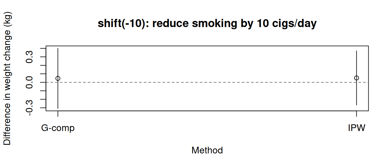
threshold() is not supported under IPW because the pushforward of a continuous density under a boundary clamp is a mixed measure (point masses at the bounds plus continuous density in the interior). Use estimator = "gcomp" for threshold interventions.
For integer-valued count treatments, pass propensity_family = "poisson" or "negbin" to use a count density model instead of the default Gaussian.
DGM. A Poisson-distributed count treatment (e.g. number of clinic visits) confounded by \(L\), with a linear outcome model.
\[ \begin{aligned} L &\sim N(0,1) \\ A &\sim \text{Poisson}\!\bigl(\exp(0.5\,L)\bigr) \\ Y &= 2 + 1.5\,A + L + \varepsilon, \quad \varepsilon \sim N(0,1) \end{aligned} \]
True contrast: \(\mathbb{E}[Y(A+1)] - \mathbb{E}[Y(A)] = 1.5\).
set.seed(6)
n <- 3000
L <- rnorm(n)
A <- rpois(n, exp(0.5 * L))
Y <- 2 + 1.5 * A + L + rnorm(n)
count_df <- data.frame(Y = Y, A = A, L = L)

fit_pois <- causat(
  count_df,
  outcome = "Y",
  treatment = "A",
  confounders = ~ L,
  estimator = "ipw",
  propensity_family = "poisson",
  model_fn = stats::glm,
  propensity_model_fn = stats::glm
)

res_pois <- contrast(
  fit_pois,
  interventions = list(plus1 = shift(1), observed = NULL),
  reference = "observed",
  type = "difference"
)
res_pois
Estimator: ipw · Estimand: ATE · Contrast: difference · CI method: sandwich · N: 3000
| intervention | estimate | se | ci_lower | ci_upper |
|---|---|---|---|---|
| plus1 | 5.267 | 0.069 | 5.133 | 5.402 |
| observed | 3.692 | 0.049 | 3.595 | 3.788 |
| comparison | estimate | se | ci_lower | ci_upper |
|---|---|---|---|---|
| plus1 vs observed | 1.576 | 0.05 | 1.478 | 1.674 |
The shift delta must be integer — shift(0.5) on a count treatment aborts because dpois() returns 0 at non-integer arguments.
scale_by() — multiply observed treatment by a factorA proportional MTP. scale_by(0.5) halves each individual’s exposure; scale_by(2) doubles it.
res_scale_gc <- contrast(
  fit_gc_cont,
  interventions = list(halved = scale_by(0.5), observed = NULL),
  reference = "observed",
  type = "difference"
)
res_scale_gc
Estimator: gcomp · Estimand: ATE · Contrast: difference · CI method: sandwich · N: 1566
| intervention | estimate | se | ci_lower | ci_upper |
|---|---|---|---|---|
| halved | 2.686 | 0.259 | 2.178 | 3.193 |
| observed | 2.638 | 0.199 | 2.248 | 3.028 |
| comparison | estimate | se | ci_lower | ci_upper |
|---|---|---|---|---|
| halved vs observed | 0.047 | 0.185 | -0.316 | 0.411 |
Under IPW, scale_by(c) evaluates the density at A / c and includes the Jacobian |1/c| in the density-ratio weight.
res_scale_ipw <- contrast(
  fit_ipw_cont,
  interventions = list(halved = scale_by(0.5), observed = NULL),
  reference = "observed",
  type = "difference"
)
res_scale_ipw
Estimator: ipw · Estimand: ATE · Contrast: difference · CI method: sandwich · N: 1566
| intervention | estimate | se | ci_lower | ci_upper |
|---|---|---|---|---|
| halved | 2.45 | 0.291 | 1.88 | 3.021 |
| observed | 2.638 | 0.199 | 2.248 | 3.028 |
| comparison | estimate | se | ci_lower | ci_upper |
|---|---|---|---|---|
| halved vs observed | -0.188 | 0.223 | -0.625 | 0.249 |
threshold() — clamp treatment within bounds (g-comp only)Caps treatment at a ceiling and/or floor. threshold(0, 20) means “nobody smokes more than 20 cigarettes per day; those below 0 are set to 0”.
res_thresh <- contrast(
  fit_gc_cont,
  interventions = list(cap20 = threshold(0, 20), observed = NULL),
  reference = "observed",
  type = "difference"
)
res_thresh
Estimator: gcomp · Estimand: ATE · Contrast: difference · CI method: sandwich · N: 1566
| intervention | estimate | se | ci_lower | ci_upper |
|---|---|---|---|---|
| cap20 | 2.659 | 0.208 | 2.252 | 3.066 |
| observed | 2.638 | 0.199 | 2.248 | 3.028 |
| comparison | estimate | se | ci_lower | ci_upper |
|---|---|---|---|---|
| cap20 vs observed | 0.021 | 0.08 | -0.137 | 0.178 |
This intervention is only available under g-computation. Under IPW, the density-ratio weight is not well-defined at the boundary clamp points (point-mass discontinuity in the pushforward density). causatr rejects threshold() under estimator = "ipw" with an informative error pointing at g-comp.
dynamic() — deterministic treatment ruleA dynamic intervention assigns treatment based on individual characteristics. The rule function receives two arguments — the full data and the observed treatment vector — and returns a vector of counterfactual treatment values.
Assign quitting only to heavy smokers (> 20 cigarettes/day at baseline):
res_dyn_gc <- contrast(
  fit_gc,
  interventions = list(
    rule = dynamic(\(data, trt) ifelse(data$smokeintensity > 20, 1, 0)),
    all_quit = static(1)
  ),
  reference = "all_quit",
  type = "difference"
)
res_dyn_gc
Estimator: gcomp · Estimand: ATE · Contrast: difference · CI method: sandwich · N: 1566
| intervention | estimate | se | ci_lower | ci_upper |
|---|---|---|---|---|
| rule | 2.725 | 0.204 | 2.325 | 3.124 |
| all_quit | 5.21 | 0.421 | 4.384 | 6.035 |
| comparison | estimate | se | ci_lower | ci_upper |
|---|---|---|---|---|
| rule vs all_quit | -2.485 | 0.337 | -3.146 | -1.824 |
Under IPW, dynamic() on a binary treatment uses Horwitz–Thompson indicator weights: w_i = I(A_i = rule_i) / f(A_i | L_i). This is well-defined because the treatment takes only two values and each individual’s counterfactual is deterministic.
res_dyn_ipw <- contrast(
  fit_ipw,
  interventions = list(
    rule = dynamic(\(data, trt) ifelse(data$smokeintensity > 20, 1, 0)),
    all_quit = static(1)
  ),
  reference = "all_quit",
  type = "difference"
)
res_dyn_ipw
Estimator: ipw · Estimand: ATE · Contrast: difference · CI method: sandwich · N: 1566
| intervention | estimate | se | ci_lower | ci_upper |
|---|---|---|---|---|
| rule | 2.803 | 0.355 | 2.107 | 3.499 |
| all_quit | 5.288 | 0.447 | 4.412 | 6.163 |
| comparison | estimate | se | ci_lower | ci_upper |
|---|---|---|---|---|
| rule vs all_quit | -2.485 | 0.385 | -3.239 | -1.73 |
Dynamic rules on continuous treatments work under g-comp (predict-then-average on the outcome model). Here, heavy smokers are reduced to 20 while others keep their observed level:
res_dyn_cont <- contrast(
  fit_gc_cont,
  interventions = list(
    capped = dynamic(\(data, trt) pmin(trt, 20)),
    observed = NULL
  ),
  reference = "observed",
  type = "difference"
)
res_dyn_cont
Estimator: gcomp · Estimand: ATE · Contrast: difference · CI method: sandwich · N: 1566
| intervention | estimate | se | ci_lower | ci_upper |
|---|---|---|---|---|
| capped | 2.659 | 0.208 | 2.252 | 3.066 |
| observed | 2.638 | 0.199 | 2.248 | 3.028 |
| comparison | estimate | se | ci_lower | ci_upper |
|---|---|---|---|---|
| capped vs observed | 0.021 | 0.08 | -0.137 | 0.178 |
dynamic() on continuous treatment is not supported under IPW. A deterministic rule on a continuous treatment is a Dirac per individual, which has no Lebesgue density — the density ratio is not defined. Rewrite the rule as a smooth shift() or scale_by(), or use estimator = "gcomp".
ipsi() — incremental propensity score intervention (IPW only)Kennedy (2019)’s incremental propensity score intervention multiplies each individual’s odds of treatment by delta. It is a stochastic MTP that never materialises a specific counterfactual treatment value — instead, it shifts the entire propensity score distribution.
The closed-form weight is: \[w_i = \frac{\delta \cdot A_i + (1 - A_i)}{\delta \cdot p_i + (1 - p_i)}\]
where \(p_i = P(A = 1 \mid L_i)\) is the fitted propensity.
IPSI is binary-treatment, IPW-only — g-comp and matching cannot evaluate it because there is no counterfactual treatment column to predict at.
res_ipsi_2 <- contrast(
  fit_ipw,
  interventions = list(double_odds = ipsi(2), natural = NULL),
  reference = "natural",
  type = "difference"
)
res_ipsi_2
Estimator: ipw · Estimand: ATE · Contrast: difference · CI method: sandwich · N: 1566
| intervention | estimate | se | ci_lower | ci_upper |
|---|---|---|---|---|
| double_odds | 3.125 | 0.218 | 2.697 | 3.552 |
| natural | 2.638 | 0.199 | 2.248 | 3.028 |
| comparison | estimate | se | ci_lower | ci_upper |
|---|---|---|---|---|
| double_odds vs natural | 0.486 | 0.066 | 0.357 | 0.615 |
res_ipsi_half <- contrast(
  fit_ipw,
  interventions = list(half_odds = ipsi(0.5), natural = NULL),
  reference = "natural",
  type = "difference"
)
res_ipsi_half
Estimator: ipw · Estimand: ATE · Contrast: difference · CI method: sandwich · N: 1566
| intervention | estimate | se | ci_lower | ci_upper |
|---|---|---|---|---|
| half_odds | 2.284 | 0.197 | 1.898 | 2.669 |
| natural | 2.638 | 0.199 | 2.248 | 3.028 |
| comparison | estimate | se | ci_lower | ci_upper |
|---|---|---|---|---|
| half_odds vs natural | -0.355 | 0.051 | -0.455 | -0.255 |
Varying delta traces out a dose-response curve on the odds scale:
deltas <- c(0.25, 0.5, 1, 2, 4)
ipsi_results <- lapply(deltas, function(d) {
  res <- contrast(
    fit_ipw,
    interventions = list(shifted = ipsi(d), natural = NULL),
    reference = "natural",
    type = "difference"
  )
  data.frame(
    delta = d,
    estimate = res$contrasts$estimate[1],
    ci_lower = res$contrasts$ci_lower[1],
    ci_upper = res$contrasts$ci_upper[1]
  )
})
ipsi_df <- do.call(rbind, ipsi_results)

tinyplot(
  estimate ~ delta,
  data = ipsi_df,
  type = "pointrange",
  ymin = ipsi_df$ci_lower,
  ymax = ipsi_df$ci_upper,
  xlab = expression(delta ~ "(odds multiplier)"),
  ylab = "E[Y(IPSI)] - E[Y(natural)] (kg)",
  main = "IPSI dose-response: effect on weight change"
)
abline(h = 0, lty = 2, col = "grey40")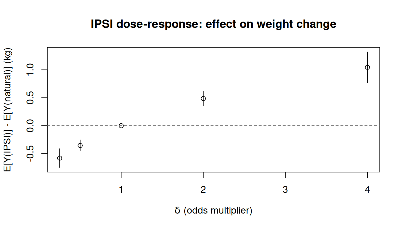
At delta = 1 the intervention is the natural course, so the contrast is zero. Larger delta makes quitting more likely and the effect on weight gain grows.
stochastic() — user-defined randomised intervention (g-comp only)A stochastic intervention draws each individual’s counterfactual treatment from a user-supplied distribution that may depend on covariates. Unlike dynamic(), which assigns a single deterministic value, stochastic() integrates over the randomness by Monte Carlo: the g-formula is evaluated n_mc times, each with an independent draw from the sampler, and the predictions are averaged.
The sampler function has the same signature as a dynamic() rule — function(data, treatment) — but should return an independent random draw each time it is called.
Assign quitting with probability that depends on smoking intensity:
set.seed(42)
res_stoch <- contrast(
  fit_gc,
  interventions = list(
    random_quit = stochastic(
      \(data, trt) rbinom(nrow(data), 1,
                          plogis(-1 + 0.05 * data$smokeintensity)),
      n_mc = 200L
    ),
    all_quit = static(1)
  ),
  reference = "all_quit",
  type = "difference"
)
res_stoch
Estimator: gcomp · Estimand: ATE · Contrast: difference · CI method: sandwich · N: 1566
| intervention | estimate | se | ci_lower | ci_upper |
|---|---|---|---|---|
| random_quit | 3.489 | 0.242 | 3.014 | 3.963 |
| all_quit | 5.21 | 0.421 | 4.384 | 6.035 |
| comparison | estimate | se | ci_lower | ci_upper |
|---|---|---|---|---|
| random_quit vs all_quit | -1.721 | 0.232 | -2.176 | -1.266 |
The estimate is a population average over both individuals and the stochastic policy.
Add a random perturbation (rather than a fixed shift) to each individual’s smoking intensity:
set.seed(42)
res_stoch_cont <- contrast(
  fit_gc_cont,
  interventions = list(
    noisy_reduce = stochastic(
      \(data, trt) trt + rnorm(length(trt), mean = -5, sd = 2),
      n_mc = 200L
    ),
    observed = NULL
  ),
  reference = "observed",
  type = "difference"
)
res_stoch_cont
Estimator: gcomp · Estimand: ATE · Contrast: difference · CI method: sandwich · N: 1566
| intervention | estimate | se | ci_lower | ci_upper |
|---|---|---|---|---|
| noisy_reduce | 2.661 | 0.211 | 2.248 | 3.074 |
| observed | 2.638 | 0.199 | 2.248 | 3.028 |
| comparison | estimate | se | ci_lower | ci_upper |
|---|---|---|---|---|
| noisy_reduce vs observed | 0.023 | 0.09 | -0.154 | 0.2 |
Choosing n_mc: 100–500 is typical. The sandwich SE accounts for the MC draws used at estimation time, so there is no need to inflate n_mc just for inference. If point estimates visibly change when you re-run with a different seed, increase n_mc.
stochastic() is only supported under estimator = "gcomp" (point and longitudinal). IPW and matching cannot evaluate it because the density ratio of a user-defined stochastic policy is generally intractable.
NULL — the natural courseNULL means “do not intervene; use the observed treatment values”. It is the natural reference for MTPs:
res_multi <- contrast(
  fit_gc_cont,
  interventions = list(
    reduce10 = shift(-10),
    halved   = scale_by(0.5),
    cap20    = threshold(0, 20),
    observed = NULL
  ),
  reference = "observed",
  type = "difference"
)
res_multi
Estimator: gcomp · Estimand: ATE · Contrast: difference · CI method: sandwich · N: 1566
| intervention | estimate | se | ci_lower | ci_upper |
|---|---|---|---|---|
| reduce10 | 2.684 | 0.256 | 2.183 | 3.186 |
| halved | 2.686 | 0.259 | 2.178 | 3.193 |
| cap20 | 2.659 | 0.208 | 2.252 | 3.066 |
| observed | 2.638 | 0.199 | 2.248 | 3.028 |
| comparison | estimate | se | ci_lower | ci_upper |
|---|---|---|---|---|
| reduce10 vs observed | 0.046 | 0.181 | -0.308 | 0.4 |
| halved vs observed | 0.047 | 0.185 | -0.316 | 0.411 |
| cap20 vs observed | 0.021 | 0.08 | -0.137 | 0.178 |
Both g-comp and IPW support multiple interventions in a single contrast() call. All pairwise differences against the reference are computed, and the variance-covariance matrix covers all interventions jointly.
est <- res_multi$contrasts
tinyplot(
  estimate ~ comparison,
  data = est,
  type = "pointrange",
  ymin = est$ci_lower,
  ymax = est$ci_upper,
  xlab = "Comparison",
  ylab = "Difference in weight change (kg)",
  main = "Multiple interventions (g-comp)"
)
abline(h = 0, lty = 2, col = "grey40")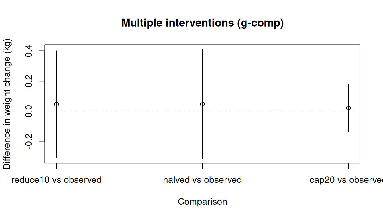
res_multi_ipw <- contrast(
  fit_ipw_cont,
  interventions = list(
    reduce10 = shift(-10),
    halved   = scale_by(0.5),
    observed = NULL
  ),
  reference = "observed",
  type = "difference"
)
res_multi_ipw
Estimator: ipw · Estimand: ATE · Contrast: difference · CI method: sandwich · N: 1566
| intervention | estimate | se | ci_lower | ci_upper |
|---|---|---|---|---|
| reduce10 | 2.69 | 0.248 | 2.205 | 3.175 |
| halved | 2.45 | 0.291 | 1.88 | 3.021 |
| observed | 2.638 | 0.199 | 2.248 | 3.028 |
| comparison | estimate | se | ci_lower | ci_upper |
|---|---|---|---|---|
| reduce10 vs observed | 0.051 | 0.163 | -0.268 | 0.371 |
| halved vs observed | -0.188 | 0.223 | -0.625 | 0.249 |
The table below summarises which combinations are supported and which are rejected with an informative error. The restrictions reflect genuine architectural limits of the density-ratio framework, not implementation gaps.
| Intervention | G-comp (point) | G-comp (longitudinal) | IPW | AIPW | Matching |
|---|---|---|---|---|---|
static() |
All treatment types | All treatment types | Binary, categorical | All types | Binary only |
shift() |
Continuous | Continuous | Continuous, count (integer delta) | Continuous | — |
scale_by() |
Continuous | Continuous | Continuous, count (integer-preserving) | Continuous | — |
threshold() |
Continuous | Continuous | — (mixed pushforward) | — | — |
dynamic() |
All treatment types | All treatment types | Binary, categorical | All types | — |
ipsi() |
— | — | Binary only | — | — |
stochastic() |
All treatment types | All treatment types | — (intractable density ratio) | — | — |
NULL |
All | All | All | All | — |
Why some combinations are rejected:
threshold() under IPW: The pushforward of a continuous density under a boundary clamp is a mixed measure — point masses at lo/hi plus continuous density in the interior. The density ratio is not well-defined.dynamic() on continuous treatment under IPW: A deterministic rule on a continuous treatment is a Dirac per individual with no Lebesgue density.static(v) on continuous treatment under IPW: Nobody is observed exactly at v, so the HT indicator I(A = v) is zero almost surely.ipsi() under g-comp/matching: IPSI shifts the propensity, not the treatment value. There is no counterfactual treatment column to predict at.stochastic() under IPW/matching: The density ratio of an arbitrary user-defined stochastic policy is generally intractable. Only g-computation (Monte Carlo integration) supports it.static() / dynamic() / threshold() / ipsi() on count treatments: Count treatments (enabled via propensity_family = "poisson" or "negbin") use dpois() / dnbinom() for the density ratio. static() is degenerate (HT indicator is zero almost surely on a count distribution). dynamic() has the same Dirac problem as on continuous. threshold() has the same mixed- measure problem. ipsi() is Bernoulli-specific. Only shift() (integer delta) and scale_by() (where A / factor is integer for every observation) are well-defined.