---
title: "Methodological triangulation: g-computation, IPW, AIPW, matching, and SNM"
code-fold: show
code-tools: true
vignette: >
%\VignetteIndexEntry{Methodological triangulation: g-computation, IPW, AIPW, matching, and SNM}
%\VignetteEngine{quarto::html}
%\VignetteEncoding{UTF-8}
bibliography: references.bib
---
```{r}
#| include: false
knitr::opts_chunk$set(collapse = TRUE, comment = "#>")
```
When multiple estimation methods agree on the same causal effect, we gain
confidence that the result is not an artefact of a single modelling assumption.
This vignette compares all five methods on the NHEFS dataset:
- **G-computation** relies on a correct outcome model.
- **IPW** relies on a correct propensity model.
- **AIPW** (doubly robust) is consistent if *either* model is correct, and
semiparametrically efficient when both are.
- **SNM** (structural nested mean model) relies on a correct treatment model
and estimates blip parameters directly — the only method that correctly
handles time-varying effect modification. See `vignette("snm")`.
- **Matching** relies on a correct propensity model and targets the ATT.
## Data: NHEFS
All examples use the **NHEFS** dataset [@hernan_whatif]. The
assumed causal structure is:
- **Treatment ($A$):** `qsmk` — quit smoking between 1971 and 1982 (binary: 0/1).
- **Outcome ($Y$):** `wt82_71` — weight change in kg (continuous), or
`gained_weight` ($\mathbf{1}\{Y > 0\}$, binary).
- **Confounders ($L$):** sex, age, race, education, smoking intensity,
years smoked, exercise, physical activity, and baseline weight.
$$
\begin{aligned}
L &\sim F_L \\
A &\sim \text{Bernoulli}\!\bigl(\text{logit}^{-1}(\alpha_0 + \alpha_L^\top L)\bigr) \\
Y &= \beta_0 + \beta_A A + \beta_L^\top L + \varepsilon
\end{aligned}
$$
The confounders $L$ are common causes of both $A$ and $Y$. Under this
structure, g-computation adjusts for $L$ via an outcome model,
IPW adjusts via a treatment model, and matching balances $L$ between
treatment groups. When all four methods agree, the result is unlikely to
be an artefact of a single modelling assumption.
```{r}
#| message: false
library(causatr)
library(tinyplot)
data("nhefs")

nhefs_complete <- nhefs[complete.cases(nhefs), ]
nhefs_complete$gained_weight <- as.integer(nhefs_complete$wt82_71 > 0)
nhefs_complete$sex <- factor(
  nhefs_complete$sex,
  levels = 0:1,
  labels = c("Male", "Female")
)

confounders <- ~ sex + age + I(age^2) + race + factor(education) +
  smokeintensity + I(smokeintensity^2) + smokeyrs + I(smokeyrs^2) +
  factor(exercise) + factor(active) + wt71 + I(wt71^2)
```
## Continuous outcome: weight change
### Fitting all four methods
```{r}
fit_gc <- causat(
  nhefs,
  outcome = "wt82_71",
  treatment = "qsmk",
  confounders = confounders,
  censoring = "censored",
  model_fn = stats::glm
)

fit_ipw <- causat(
  nhefs_complete,
  outcome = "wt82_71",
  treatment = "qsmk",
  confounders = confounders,
  estimator = "ipw",
  model_fn = stats::glm,
  propensity_model_fn = stats::glm
)

fit_aipw <- causat(
  nhefs_complete,
  outcome = "wt82_71",
  treatment = "qsmk",
  confounders = confounders,
  estimator = "aipw",
  model_fn = stats::glm,
  propensity_model_fn = stats::glm
)

fit_m <- causat(
  nhefs_complete,
  outcome = "wt82_71",
  treatment = "qsmk",
  confounders = confounders,
  estimator = "matching",
  estimand = "ATT"
)
```
### Contrasts
```{r}
ivs <- list(quit = static(1), continue = static(0))
res_gc <- contrast(fit_gc, ivs, reference = "continue")
res_ipw <- contrast(fit_ipw, ivs, reference = "continue")
res_aipw <- contrast(fit_aipw, ivs, reference = "continue")
res_m <- contrast(fit_m, ivs, reference = "continue")
results <- rbind(
cbind(method = "G-computation", res_gc$contrasts),
cbind(method = "IPW", res_ipw$contrasts),
cbind(method = "AIPW", res_aipw$contrasts),
cbind(method = "Matching (ATT)", res_m$contrasts)
)
results
```
::: {.callout-note}
## Why AIPW SE may be smaller
When both the outcome and propensity models are correctly specified, AIPW
attains the semiparametric efficiency bound — its standard error is no larger
than either plain g-computation or plain IPW. In applied data the gain is
often modest but never negative.
:::
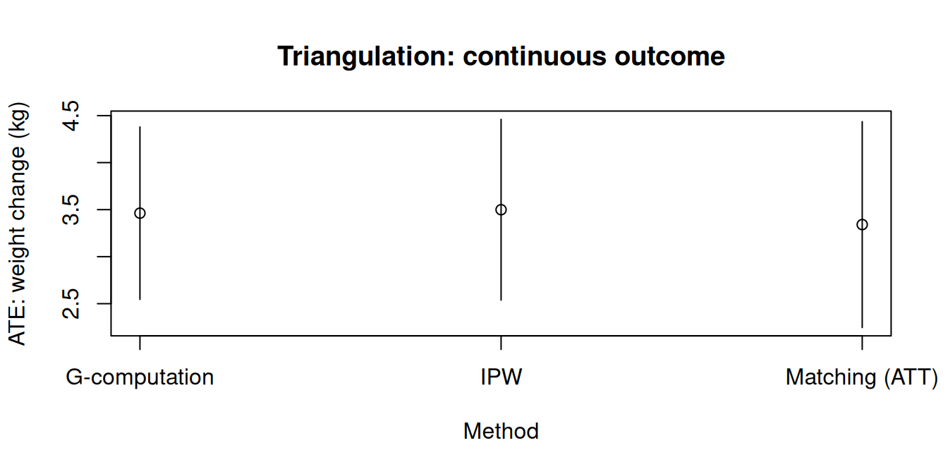
### Forest plot
```{r}
#| fig-width: 7
#| fig-height: 4
#| fig-alt: "Forest plot comparing g-computation, IPW, AIPW, and matching estimates of the effect of quitting smoking on weight change."
tinyplot(
  estimate ~ method,
  data = results,
  type = "pointrange",
  ymin = results$ci_lower,
  ymax = results$ci_upper,
  xlab = "Method",
  ylab = "ATE: weight change (kg)",
  main = "Triangulation: continuous outcome"
)
abline(h = 0, lty = 2, col = "grey40")
```
## Binary outcome: gained weight
```{r}
fit_gc_bin <- causat(
nhefs_complete,
outcome = "gained_weight",
treatment = "qsmk",
confounders = confounders,
family = "binomial",
model_fn = stats::glm
)
fit_ipw_bin <- causat(
nhefs_complete,
outcome = "gained_weight",
treatment = "qsmk",
confounders = confounders,
estimator = "ipw",
model_fn = stats::glm,
propensity_model_fn = stats::glm
)
fit_aipw_bin <- causat(
nhefs_complete,
outcome = "gained_weight",
treatment = "qsmk",
confounders = confounders,
estimator = "aipw",
family = "binomial",
model_fn = stats::glm,
propensity_model_fn = stats::glm
)
fit_m_bin <- causat(
nhefs_complete,
outcome = "gained_weight",
treatment = "qsmk",
confounders = confounders,
estimator = "matching",
estimand = "ATT"
)
res_gc_bin <- contrast(fit_gc_bin, ivs, reference = "continue")
res_ipw_bin <- contrast(fit_ipw_bin, ivs, reference = "continue")
res_aipw_bin <- contrast(fit_aipw_bin, ivs, reference = "continue")
res_m_bin <- contrast(fit_m_bin, ivs, reference = "continue")
results_bin <- rbind(
cbind(method = "G-computation", res_gc_bin$contrasts),
cbind(method = "IPW", res_ipw_bin$contrasts),
cbind(method = "AIPW", res_aipw_bin$contrasts),
cbind(method = "Matching (ATT)", res_m_bin$contrasts)
)
results_bin
```
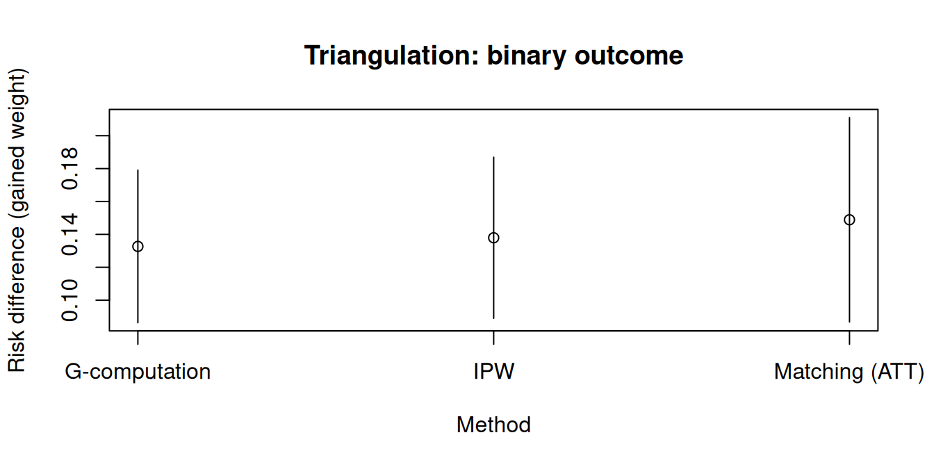
```{r}
#| fig-width: 7
#| fig-height: 4
#| fig-alt: "Forest plot comparing g-computation, IPW, AIPW, and matching on the binary outcome (gained weight)."
tinyplot(
  estimate ~ method,
  data = results_bin,
  type = "pointrange",
  ymin = results_bin$ci_lower,
  ymax = results_bin$ci_upper,
  xlab = "Method",
  ylab = "Risk difference (gained weight)",
  main = "Triangulation: binary outcome"
)
abline(h = 0, lty = 2, col = "grey40")
```
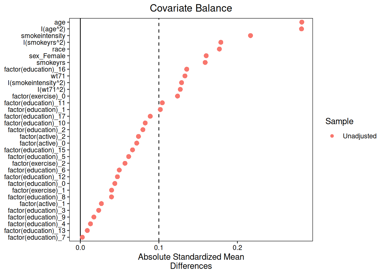
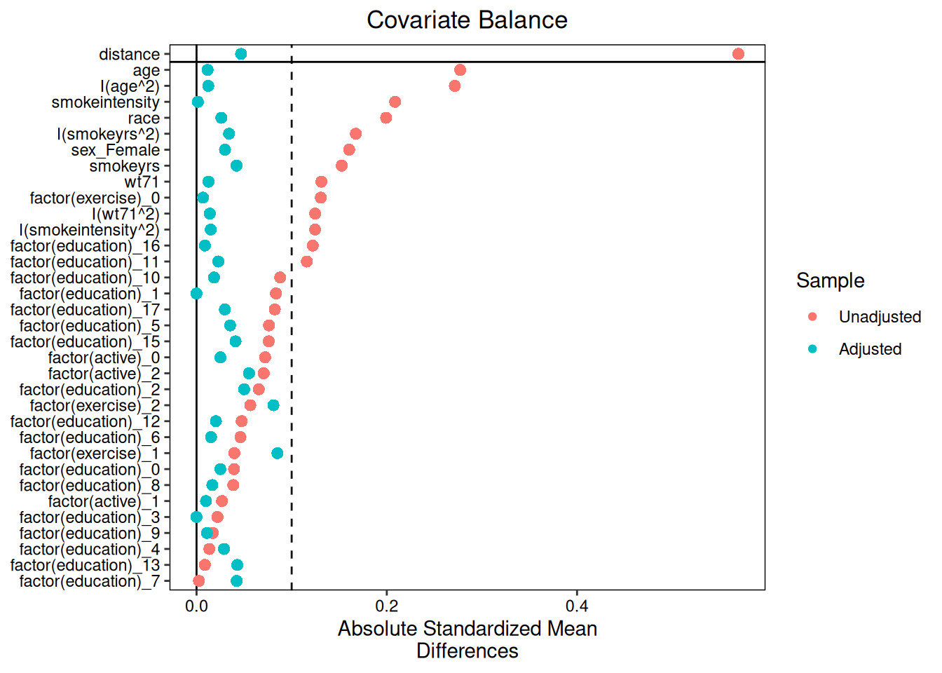
## Diagnostics
Before interpreting results, check that the assumptions hold. `diagnose()`
provides positivity checks, covariate balance, and method-specific summaries.
```{r}
diag_ipw <- diagnose(fit_ipw)
diag_m <- diagnose(fit_m)
```
### IPW balance
```{r}
#| fig-width: 7
#| fig-height: 5
#| fig-alt: "Love plot for IPW covariate balance in the triangulation analysis."
plot(diag_ipw)
```
### Matching balance
```{r}
#| fig-width: 7
#| fig-height: 5
#| fig-alt: "Love plot for matching covariate balance in the triangulation analysis."
plot(diag_m)
```
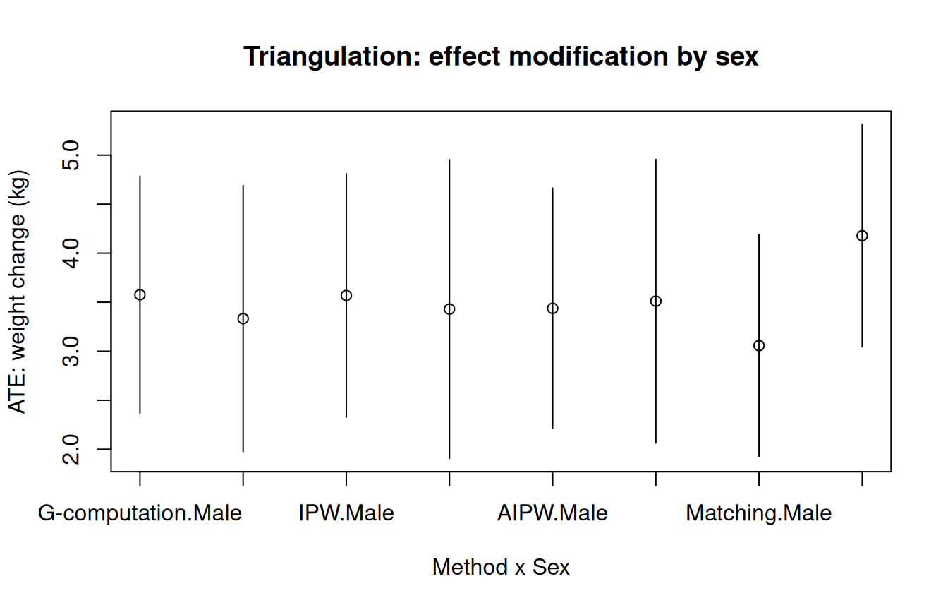
## Cross-method effect modification
All four point-treatment methods support effect modification via
`A:modifier` interaction terms in `confounders`. When the four methods
agree on stratum-specific treatment effects, this gives strong evidence
that the effect heterogeneity is real rather than an artefact of model
specification.
Here we add `qsmk:sex` to examine whether the effect of quitting smoking
on weight change differs by sex. Each method handles the interaction
differently (g-comp feeds it to the outcome model; IPW expands the MSM to
`Y ~ 1 + sex`; matching expands to `Y ~ qsmk + sex + qsmk:sex`), but all
should recover the same stratum-specific estimates under correct
specification.
```{r}
confounders_em <- ~ sex + age + I(age^2) + race + factor(education) +
smokeintensity + I(smokeintensity^2) + smokeyrs + I(smokeyrs^2) +
factor(exercise) + factor(active) + wt71 + I(wt71^2) +
qsmk:sex
fit_gc_em <- causat(
nhefs_complete,
outcome = "wt82_71",
treatment = "qsmk",
confounders = confounders_em,
model_fn = stats::glm
)
fit_ipw_em <- causat(
nhefs_complete,
outcome = "wt82_71",
treatment = "qsmk",
confounders = confounders_em,
estimator = "ipw",
model_fn = stats::glm,
propensity_model_fn = stats::glm
)
fit_aipw_em <- causat(
nhefs_complete,
outcome = "wt82_71",
treatment = "qsmk",
confounders = confounders_em,
estimator = "aipw",
model_fn = stats::glm,
propensity_model_fn = stats::glm
)
fit_m_em <- causat(
nhefs_complete,
outcome = "wt82_71",
treatment = "qsmk",
confounders = confounders_em,
estimator = "matching"
)
res_gc_em <- contrast(
fit_gc_em, ivs,
reference = "continue",
ci_method = "sandwich",
by = "sex"
)
res_ipw_em <- contrast(
fit_ipw_em, ivs,
reference = "continue",
ci_method = "sandwich",
by = "sex"
)
res_aipw_em <- contrast(
fit_aipw_em, ivs,
reference = "continue",
ci_method = "sandwich",
by = "sex"
)
res_m_em <- contrast(
fit_m_em, ivs,
reference = "continue",
ci_method = "sandwich",
by = "sex"
)
results_em <- rbind(
cbind(method = "G-computation", res_gc_em$contrasts),
cbind(method = "IPW", res_ipw_em$contrasts),
cbind(method = "AIPW", res_aipw_em$contrasts),
cbind(method = "Matching", res_m_em$contrasts)
)
results_em
```
```{r}
#| fig-width: 7
#| fig-height: 4.5
#| fig-alt: "Forest plot comparing g-computation, IPW, AIPW, and matching on sex-stratified ATE."
tinyplot(
  estimate ~ interaction(method, by),
  data = results_em,
  type = "pointrange",
  ymin = results_em$ci_lower,
  ymax = results_em$ci_upper,
  xlab = "Method x Sex",
  ylab = "ATE: weight change (kg)",
  main = "Triangulation: effect modification by sex"
)
abline(h = 0, lty = 2, col = "grey40")
```
Agreement across methods within each stratum provides evidence that the
sex-specific effects are real. Disagreement would point to model
misspecification in one or more methods.
::: {.callout-important}
## Effect modifier must be a baseline variable under IPW, AIPW, and matching
Under IPW, AIPW, and matching, the modifier in `A:modifier` must be a
**baseline** (pre-treatment) variable. A time-varying modifier in a marginal
structural model conditions on a post-treatment variable, which biases the
estimand via mediator and collider paths [@robins2000msmepi].
G-computation has no such restriction because it models the outcome, not
the treatment.
For **time-varying effect modification** (modifiers affected by prior
treatment), use `estimator = "snm"` — see `vignette("snm")`.
causatr does not enforce baseline-ness at runtime (time-varying status isn't
inferable from data alone). This is a user responsibility.
:::
## When to use which method
| Criterion | G-computation | IPW | AIPW | SNM | Matching |
|---|---|---|---|---|---|
| Model required | Outcome | Treatment | Both | Treatment | Treatment |
| Doubly robust | No | No | **Yes** | No | No |
| Semiparametrically efficient | No | No | **Yes** (when both correct) | No | No |
| Non-static interventions | Yes | Yes (shift, scale\_by, dynamic, IPSI) | Yes (same as IPW) | No (`treatment_values =` only) | No (static only) |
| Continuous treatment | Yes | Yes (GPS) | Yes (shift, scale\_by) | Yes | No |
| Categorical (k > 2) | Yes | Yes | Yes | Pending | No |
| Longitudinal (time-varying) | Yes (ICE) | Yes | Yes (ICE-AIPW) | Yes (backward g-estimation) | No |
| Time-varying effect modification | Requires correct high-dim outcome model | Biased | Biased | **Yes** (headline use case) | Biased |
| Variance estimation | Sandwich or bootstrap | Sandwich or bootstrap | Sandwich or bootstrap | Sandwich (bootstrap pending) | Cluster-robust sandwich |
**Recommendation:**
- Use **AIPW** when you have credible models for both the outcome and treatment
and want protection against misspecification in either one.
- Use **g-computation** when you want to exploit complex outcome-model
structure (e.g. `threshold()` interventions, GAM nuisances) not supported
by the density-ratio engine.
- Use **IPW** when the treatment model is the primary scientific object and
you want to avoid specifying an outcome model.
- Use **SNM** when your research question involves effect modification by a
variable that is itself affected by treatment — the other methods produce
biased results in this setting. See `vignette("snm")`.
- Use **matching** for ATT estimation with balance diagnostics as the primary
product.
When all methods agree, the result is unlikely to be an artefact of any
single modelling assumption. Disagreement points to misspecification — investigate
further with `diagnose()` and covariate balance checks.
For features marked "No", causatr aborts at fit or contrast time with a
pointer to the planning doc rather than silently returning a wrong answer —
see `FEATURE_COVERAGE_MATRIX.md` for the full rejection-path inventory.
## Separate confounders for double robustness
AIPW is consistent when *either* the outcome model or the propensity
model is correctly specified. To exploit this, you can pass different
covariate sets to each model via `confounders_outcome` and
`confounders_treatment`:
```{r}
#| eval: false
fit_dr <- causat(
  nhefs_complete,
  outcome = "wt82_71",
  treatment = "qsmk",
  confounders_outcome = ~ sex + age + I(age^2) + race +
    factor(education) + smokeintensity + I(smokeintensity^2) +
    smokeyrs + I(smokeyrs^2) + factor(exercise) + factor(active) +
    wt71 + I(wt71^2),
  confounders_treatment = ~ sex + age + race + factor(education) +
    smokeintensity + smokeyrs + factor(exercise) + factor(active) + wt71,
  estimator = "aipw",
  propensity_model_fn = stats::glm
)
```
The same per-component formulas are available for every estimator (though
g-comp only uses the outcome side and IPW only uses the treatment side).
Additional per-component formulas exist for the censoring model
(`confounders_censoring`), the transportability sampling model
(`confounders_sampling`), and time-varying confounders
(`confounders_tv_outcome`, `confounders_tv_treatment`).
The legacy `confounders` argument still works as a shorthand that sets
all components at once.
## References
::: {#refs}
:::