---
title: "Propensity score matching with causatr"
code-fold: show
code-tools: true
vignette: >
%\VignetteIndexEntry{Propensity score matching with causatr}
%\VignetteEngine{quarto::html}
%\VignetteEncoding{UTF-8}
bibliography: references.bib
---
```{r}
#| include: false
knitr::opts_chunk$set(collapse = TRUE, comment = "#>")
```
Propensity score matching estimates causal effects by pairing treated and
control individuals with similar propensity scores, then comparing outcomes
within matched sets. causatr delegates match construction to
[MatchIt](https://kosukeimai.github.io/MatchIt/) [@ho2011matchit] and fits the outcome model
on the matched sample. Inference runs through the unified influence-function
variance engine (`variance_if()`): IFs are computed on the matched sample and
aggregated **cluster-robustly** on the matched-pair subclass — the IF analogue
of `sandwich::vcovCL()`, derived in `vignettes/variance-theory.qmd` §4.3.
This vignette demonstrates propensity score matching in causatr using the NHEFS
dataset from @hernan_whatif, covering every supported combination of
treatment type, outcome type, contrast scale, and inference method for
time-fixed treatments.
**Note:** Matching supports only `static()` interventions and **binary
point treatments**. `MatchIt` itself is binary-only, so categorical
(k > 2 levels) and continuous treatments are rejected up front with a
clear error — use `estimator = "gcomp"` or `estimator = "ipw"` for those.
Longitudinal matching is also not supported. For modified treatment
policies (shift / scale / threshold / dynamic / MTP), use
g-computation (see `vignette("gcomp")`).
## Data: NHEFS
All examples use the **NHEFS** dataset [@hernan_whatif]. The
assumed causal structure is:
- **Treatment ($A$):** `qsmk` — quit smoking between 1971 and 1982 (binary: 0/1).
- **Outcome ($Y$):** `wt82_71` — weight change in kg (continuous), or
`gained_weight` ($\mathbf{1}\{Y > 0\}$, binary).
- **Confounders ($L$):** sex, age, race, education, smoking intensity,
years smoked, exercise, physical activity, and baseline weight — common
causes of both $A$ and $Y$.
Propensity score matching estimates $\mathbb{E}[Y^{a=1}] - \mathbb{E}[Y^{a=0}]$
by constructing a matched sample where the distribution of $L$ is
(approximately) balanced across treatment groups, then comparing outcomes
within matched sets.
```{r}
#| message: false
library(causatr)
library(tinytable)
library(tinyplot)

data("nhefs")

nhefs_complete <- nhefs[complete.cases(nhefs), ]

nhefs_complete$gained_weight <- as.integer(nhefs_complete$wt82_71 > 0)

nhefs_complete$sex <- factor(
  nhefs_complete$sex,
  levels = 0:1,
  labels = c("Male", "Female")
)
```
## Binary treatment, continuous outcome
Matching estimate of the effect of quitting smoking on weight change, following
the approach in Chapter 15 of @hernan_whatif.
### ATT with sandwich SE
Matching naturally targets the ATT (effect on the treated). This is the default
for nearest-neighbour matching.
```{r}
fit_m <- causat(
  nhefs_complete,
  outcome = "wt82_71",
  treatment = "qsmk",
  confounders = ~ sex + age + I(age^2) + race + factor(education) +
    smokeintensity + I(smokeintensity^2) + smokeyrs + I(smokeyrs^2) +
    factor(exercise) + factor(active) + wt71 + I(wt71^2),
  estimator = "matching",
  estimand = "ATT"
)

res_att_sw <- contrast(
  fit_m,
  interventions = list(quit = static(1), continue = static(0)),
  reference = "continue",
  type = "difference",
  ci_method = "sandwich"
)
res_att_sw
```
### ATT with bootstrap SE
The bootstrap resamples individuals, re-matches, and refits the outcome model
on each bootstrap sample, fully accounting for matching uncertainty.
```{r}
res_att_bs <- contrast(
  fit_m,
  interventions = list(quit = static(1), continue = static(0)),
  reference = "continue",
  type = "difference",
  ci_method = "bootstrap",
  n_boot = 50L
)
res_att_bs
```
### ATE estimand
For the ATE, MatchIt performs full matching (each unit gets a weight) rather
than 1:1 nearest-neighbour matching.
```{r}
#| eval: !expr requireNamespace("optmatch", quietly = TRUE)
fit_m_ate <- causat(
  nhefs_complete,
  outcome = "wt82_71",
  treatment = "qsmk",
  confounders = ~ sex + age + I(age^2) + race + factor(education) +
    smokeintensity + I(smokeintensity^2) + smokeyrs + I(smokeyrs^2) +
    factor(exercise) + factor(active) + wt71 + I(wt71^2),
  estimator = "matching",
  estimand = "ATE"
)

res_ate_sw <- contrast(
  fit_m_ate,
  interventions = list(quit = static(1), continue = static(0)),
  reference = "continue",
  type = "difference",
  ci_method = "sandwich"
)
res_ate_sw
```
### ATE with bootstrap SE
```{r}
#| eval: !expr requireNamespace("optmatch", quietly = TRUE)
res_ate_bs <- contrast(
  fit_m_ate,
  interventions = list(quit = static(1), continue = static(0)),
  reference = "continue",
  type = "difference",
  ci_method = "bootstrap",
  n_boot = 50L
)
res_ate_bs
```
### ATT with external survey weights
Pre-computed survey weights are passed via `weights =` to `causat()`
(either as a numeric vector or as a `survey::svydesign` object — the
latter is unpacked automatically) and validated upfront by
`check_weights()`. Internally causatr **multiplies** the survey weights
by the match weights from `MatchIt`; the combined weight drives the
outcome-model fit on the matched sample and enters the cluster-robust
IF variance via `prior.weights`. The row-alignment between the matched
sample and the user-supplied weights is handled by
`combine_match_and_external_weights()` (defined in `R/matching.R`) so
the invariant is asserted in exactly one place.
::: {.callout-note}
## Cluster argument not available for matching
`causat(cluster = ...)` and `contrast(cluster = ...)` are rejected with a
`causatr_bad_cluster` abort under `estimator = "matching"`. The matched
sample is already aggregated cluster-robustly on `subclass` (pair or
stratum), and a user-supplied design cluster would either conflict with
or double-count the within-subclass rows. For a design cluster outside
the matched structure (site, household, PSU), use `estimator = "gcomp"`
or `"ipw"` instead — both expose the same sum-within-cluster-then-square
IF aggregation via `cluster =`.
Similarly, passing a `survey::svydesign` object with non-trivial PSUs
to `weights =` under matching aborts: the design's first-stage cluster
would land in the cluster slot and hit the same rejection. Use
`svydesign(ids = ~1, weights = ~pw, data = d)` to declare a
sampling-weight-only design (no clustering), or supply the weights
as a numeric vector.
:::
```{r}
set.seed(42)
# Synthetic survey weights unrelated to the outcome — demonstrates the
# plumbing without introducing real bias.
svy_w <- runif(nrow(nhefs_complete), 0.5, 2.0)

fit_m_sv <- causat(
  nhefs_complete,
  outcome = "wt82_71",
  treatment = "qsmk",
  confounders = ~ sex + age + I(age^2) + race + factor(education) +
    smokeintensity + I(smokeintensity^2) + smokeyrs + I(smokeyrs^2) +
    factor(exercise) + factor(active) + wt71 + I(wt71^2),
  estimator = "matching",
  estimand = "ATT",
  weights = svy_w
)

res_m_sv <- contrast(
  fit_m_sv,
  interventions = list(quit = static(1), continue = static(0)),
  reference = "continue",
  type = "difference",
  ci_method = "sandwich"
)
res_m_sv
```
### ATC estimand
The ATC targets the effect among controls (those who continued smoking).
```{r}
fit_m_atc <- causat(
nhefs_complete,
outcome = "wt82_71",
treatment = "qsmk",
confounders = ~ sex + age + I(age^2) + race + factor(education) +
smokeintensity + I(smokeintensity^2) + smokeyrs + I(smokeyrs^2) +
factor(exercise) + factor(active) + wt71 + I(wt71^2),
estimator = "matching",
estimand = "ATC"
)
res_atc <- contrast(
fit_m_atc,
interventions = list(quit = static(1), continue = static(0)),
reference = "continue",
type = "difference",
ci_method = "sandwich"
)
res_atc
```
### Extracting results programmatically
```{r}
coef(res_att_sw)
confint(res_att_sw)
vcov(res_att_sw)
tidy(res_att_sw)
glance(res_att_sw)
```
## Binary treatment, binary outcome
Using the `gained_weight` indicator as a binary outcome. The outcome model on
the matched sample is still `Y ~ A` (linear probability model), so
`contrast()` computes marginal risks from the weighted predictions.
### Risk difference (sandwich)
```{r}
fit_m_bin <- causat(
  nhefs_complete,
  outcome = "gained_weight",
  treatment = "qsmk",
  confounders = ~ sex + age + I(age^2) + race + factor(education) +
    smokeintensity + I(smokeintensity^2) + smokeyrs + I(smokeyrs^2) +
    factor(exercise) + factor(active) + wt71 + I(wt71^2),
  estimator = "matching",
  estimand = "ATT"
)

res_rd <- contrast(
  fit_m_bin,
  interventions = list(quit = static(1), continue = static(0)),
  reference = "continue",
  type = "difference",
  ci_method = "sandwich"
)
res_rd
```
### Risk difference (bootstrap)
```{r}
res_rd_bs <- contrast(
  fit_m_bin,
  interventions = list(quit = static(1), continue = static(0)),
  reference = "continue",
  type = "difference",
  ci_method = "bootstrap",
  n_boot = 50L
)
res_rd_bs
```
### Risk ratio
```{r}
res_rr <- contrast(
  fit_m_bin,
  interventions = list(quit = static(1), continue = static(0)),
  reference = "continue",
  type = "ratio",
  ci_method = "sandwich"
)
res_rr
```
### Odds ratio
```{r}
res_or <- contrast(
  fit_m_bin,
  interventions = list(quit = static(1), continue = static(0)),
  reference = "continue",
  type = "or",
  ci_method = "sandwich"
)
res_or
```
### Risk ratio (bootstrap)
```{r}
res_rr_bs <- contrast(
  fit_m_bin,
  interventions = list(quit = static(1), continue = static(0)),
  reference = "continue",
  type = "ratio",
  ci_method = "bootstrap",
  n_boot = 50L
)
res_rr_bs
```
### Quasibinomial outcome
When binary outcomes exhibit over-dispersion or you want conservative SEs
without the strict binomial variance assumption, use `family = "quasibinomial"`:
```{r}
fit_m_quasi <- causat(
  nhefs_complete,
  outcome = "gained_weight",
  treatment = "qsmk",
  confounders = ~ sex + age + I(age^2) + race + factor(education) +
    smokeintensity + I(smokeintensity^2) + smokeyrs + I(smokeyrs^2) +
    factor(exercise) + factor(active) + wt71 + I(wt71^2),
  estimator = "matching",
  estimand = "ATT",
  family = "quasibinomial"
)

res_quasi <- contrast(
  fit_m_quasi,
  interventions = list(quit = static(1), continue = static(0)),
  reference = "continue",
  type = "difference",
  ci_method = "sandwich"
)
res_quasi
```
```{r}
tt(tidy(res_quasi), digits = 3)
```
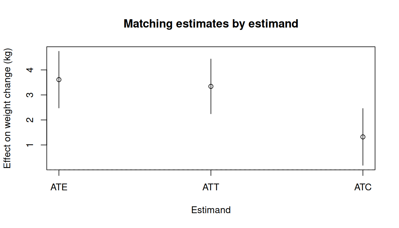
## Comparing estimands
```{r}
#| fig-width: 7
#| fig-height: 4
#| fig-alt: "Point estimates and confidence intervals for ATT and ATC (and ATE if optmatch is available) estimated by matching."
results_list <- list(
  data.frame(
    estimand = "ATT",
    estimate = res_att_sw$contrasts$estimate[1],
    ci_lower = res_att_sw$contrasts$ci_lower[1],
    ci_upper = res_att_sw$contrasts$ci_upper[1]
  ),
  data.frame(
    estimand = "ATC",
    estimate = res_atc$contrasts$estimate[1],
    ci_lower = res_atc$contrasts$ci_lower[1],
    ci_upper = res_atc$contrasts$ci_upper[1]
  )
)
if (requireNamespace("optmatch", quietly = TRUE)) {
  results_list <- c(list(data.frame(
    estimand = "ATE",
    estimate = res_ate_sw$contrasts$estimate[1],
    ci_lower = res_ate_sw$contrasts$ci_lower[1],
    ci_upper = res_ate_sw$contrasts$ci_upper[1]
  )), results_list)
}
est_df <- do.call(rbind, results_list)

tinyplot(
  estimate ~ estimand,
  data = est_df,
  type = "pointrange",
  ymin = est_df$ci_lower,
  ymax = est_df$ci_upper,
  xlab = "Estimand",
  ylab = "Effect on weight change (kg)",
  main = "Matching estimates by estimand"
)
abline(h = 0, lty = 2, col = "grey40")
```
## Forwarding MatchIt arguments (CEM)
Any extra arguments passed to `causat()` flow through `...` straight into
`MatchIt::matchit()`. Because the causatr argument is now `estimator` (not
`method`), MatchIt's own `method = "..."` is free and you can pick a
non-default matching algorithm. The example below swaps the default
nearest-neighbor matcher for **coarsened exact matching** [@iacus2012cem],
which is built into MatchIt and needs no extra packages.
Other forwardable values include `"optimal"` (needs `optmatch`),
`"genetic"` (needs `Matching`), `"cardinality"` (needs an LP solver), and
the full MatchIt method list.
```{r}
fit_cem <- causat(
  nhefs_complete,
  outcome = "wt82_71",
  treatment = "qsmk",
  confounders = ~ sex + age + race + factor(education) +
    smokeintensity + smokeyrs + factor(exercise) + factor(active) + wt71,
  estimator = "matching",
  estimand = "ATT",
  method = "cem"  # forwarded to MatchIt::matchit()
)

res_cem <- contrast(
  fit_cem,
  interventions = list(quit = static(1), continue = static(0)),
  reference = "continue",
  type = "difference",
  ci_method = "sandwich"
)
res_cem
```
Any additional MatchIt knobs (`ratio`, `replace`, `caliper`, `distance`,
`k2k`, …) can be passed the same way.
## Effect modification with `by`
When `confounders` includes an `A:modifier` interaction term, matching
expands the outcome MSM from `Y ~ A` to `Y ~ A + modifier + A:modifier`.
The saturated MSM recovers stratum-specific treatment effects on the
matched sample. Use `by = "modifier"` in `contrast()` to obtain
heterogeneous treatment effects.
Here we add a `qsmk:sex` interaction to examine how the effect of quitting
smoking on weight change differs by sex. The propensity score model used
for matching automatically strips the interaction term.
```{r}
#| eval: !expr requireNamespace("optmatch", quietly = TRUE)
fit_m_hte <- causat(
  nhefs_complete,
  outcome = "wt82_71",
  treatment = "qsmk",
  confounders = ~ sex + age + I(age^2) + race + factor(education) +
    smokeintensity + I(smokeintensity^2) + smokeyrs + I(smokeyrs^2) +
    factor(exercise) + factor(active) + wt71 + I(wt71^2) +
    qsmk:sex,
  estimator = "matching"
)

res_m_by_sex <- contrast(
  fit_m_hte,
  interventions = list(quit = static(1), continue = static(0)),
  reference = "continue",
  type = "difference",
  ci_method = "sandwich",
  by = "sex"
)
res_m_by_sex
```
::: {.callout-note}
The matching expansion differs from IPW: because matching weights are
subclass indicators (not density-ratio weights), the treatment is **not**
absorbed by the weights. The outcome MSM must therefore include `A`,
`modifier`, and `A:modifier` --- the full saturated model for the
treatment-by-modifier interaction. The propensity score model used for
match construction strips the `A:modifier` term automatically.
:::
## Tidy and glance
causatr results work with the broom ecosystem via `tidy()` and `glance()`:
```{r}
tidy(res_att_sw)
glance(res_att_sw)
```
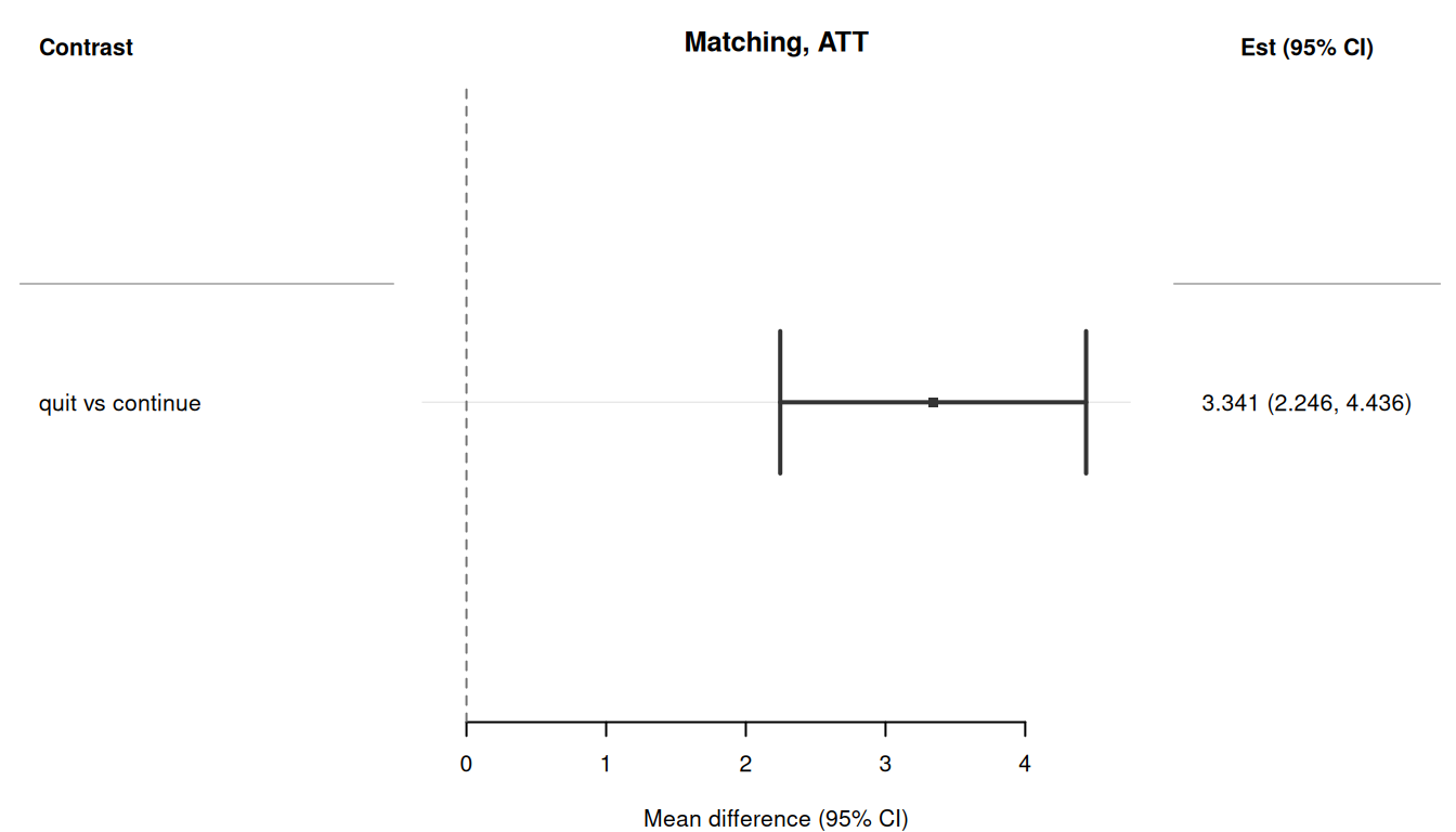
## Forest plot
The `plot()` method produces a forest plot using the `forrest` package.
```{r}
#| fig-width: 7
#| fig-height: 4
#| fig-alt: "Forest plot of the matching-estimated ATT of quitting smoking on weight change."
#| eval: !expr requireNamespace("forrest", quietly = TRUE)
plot(res_att_sw)
```
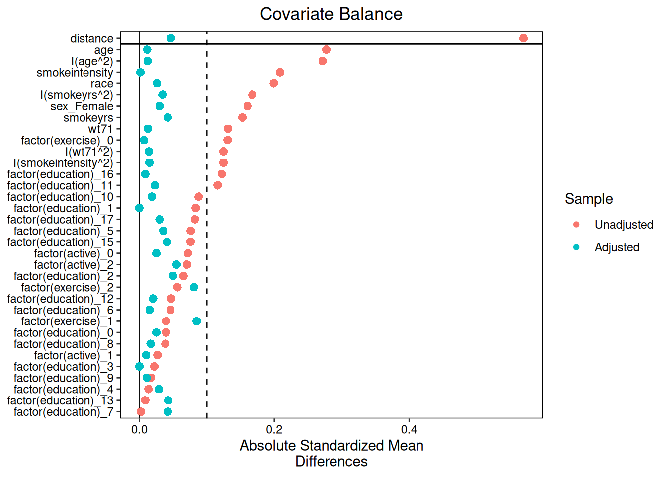
## Diagnostics
After fitting a matching model, use `diagnose()` to assess covariate balance
and match quality. Balance diagnostics use
[cobalt](https://ngreifer.github.io/cobalt/) to compare SMDs before and after
matching.
```{r}
diag <- diagnose(fit_m)
diag
```
### Love plot
```{r}
#| fig-width: 7
#| fig-height: 5
#| fig-alt: "Love plot showing covariate balance before and after propensity score matching."
plot(diag)
```
### Match quality
```{r}
diag$match_quality
```
## Summary of covered combinations
**Legend.** ✅ covered and truth-pinned in tests · 🟡 smoke test only ·
⛔ rejected with an informative error.
| Treatment | Outcome | Intervention | Estimand | Contrast | Inference | Weights | Status |
|---|---|---|---|---|---|---|---|
| Binary | Continuous | Static | ATT | Difference | Sandwich | none | ✅ |
| Binary | Continuous | Static | ATT | Difference | Bootstrap | none | ✅ |
| Binary | Continuous | Static | ATT | Difference | Sandwich | survey | ✅ |
| Binary | Continuous | Static | ATE | Difference | Sandwich | none | ✅ |
| Binary | Continuous | Static | ATE | Difference | Bootstrap | none | ✅ |
| Binary | Continuous | Static | ATC | Difference | Sandwich | none | ✅ |
| Binary | Binary | Static | ATT | Difference | Sandwich | none | ✅ |
| Binary | Binary | Static | ATT | Difference | Bootstrap | none | ✅ |
| Binary | Binary | Static | ATT | Ratio | Sandwich | none | ✅ |
| Binary | Binary | Static | ATT | OR | Sandwich | none | ✅ |
| Binary | Binary (quasibinomial) | Static | ATT | Difference | Sandwich | none | ✅ |
| Binary | Binary | Static | ATT | Ratio | Bootstrap | none | ✅ |
| Binary | Gaussian | Static | ATE (with `A:modifier`) | Difference | Sandwich / Bootstrap | none | ✅ |
| Categorical (k>2) / Continuous | — | — | — | — | — | — | ⛔ binary only |
| Any | — | Dynamic / Shift / Scale / Threshold / IPSI | — | — | — | — | ⛔ Phase 4 |
See `FEATURE_COVERAGE_MATRIX.md`
for the authoritative coverage status of every method × treatment × outcome
× intervention × variance combination.
## References
::: {#refs}
:::