Longitudinal treatments: ICE g-computation

When treatment and confounders vary over time, standard regression methods give biased estimates even when adjusted for all confounders. G-methods solve this. causatr implements ICE (iterated conditional expectation) g-computation (Zivich et al., 2024), which requires models for the outcome only — no models for time-varying confounders are needed.

Doubly-robust longitudinal estimation

For doubly-robust protection, use estimator = "aipw". ICE-AIPW (Bang & Robins 2005) augments each backward regression step with a propensity-weighted residual correction, giving a consistent estimator if either the outcome regression or the propensity model at each time point is correctly specified. The same causat() + contrast() API applies; sandwich and bootstrap variance are both supported.

This vignette demonstrates ICE g-computation in causatr, covering:

The treatment-confounder feedback problem
ICE fitting and contrasting
Sandwich and bootstrap inference
Static, dynamic, and modified treatment policy interventions
The history parameter (Markov order)
Binary outcomes
Comparison with naive regression

Setup

Code

library(causatr)
library(tinytable)
library(tinyplot)

The problem: treatment-confounder feedback

When $A_0$ affects a time-varying confounder $L_1$, and $L_1$ in turn affects both $A_1$ and $Y$ ($A_0 \to L_1 \to A_1$ and $L_1 \to Y$), ordinary regression cannot recover the marginal counterfactual mean $\mathbb{E}[Y^{a_0, a_1}]$:

Adjusting for $L_1$ blocks part of the causal path from $A_0$ to $Y$ (and, depending on the DAG, can open a collider path through unmeasured common causes of $L_1$ and $Y$).
Not adjusting leaves $L_1$-confounding of the $A_1 \to Y$ arrow.
ICE g-computation handles both correctly by iterating conditional expectations and marginalising over the $L_1$ distribution induced by each intervention.

Table 20.1: the null paradox

We reconstruct the dataset from Table 20.1 of Hernan & Robins (2025), scaled to 3,200 individuals observed at 2 time points. (The original table has 32,000; we use 1/10th for faster vignette rendering.) The DGP has a very specific property: every joint regime $(a_0, a_1)$ has the same marginal counterfactual mean $\mathbb{E}[Y^{a_0, a_1}] = 60$, so the true causal contrast between any two regimes is exactly zero — the “null is true”. Crucially, the null holds only marginally: within strata of $L_1$, the conditional effect of $A_0$ is $-8$. Treatment-confounder feedback is exactly the mechanism that lets a non-zero conditional effect average out to a zero marginal effect.

DGM. Two periods ($k = 0, 1$) with binary treatment $A_k \in \{0, 1\}$, binary time-varying confounder $L_1 \in \{0, 1\}$ (affected by $A_0$), and continuous outcome $Y$ measured at $k = 1$. The causal structure is $A_0 \to L_1 \to A_1$, $A_0 \to L_1 \to Y$, and $A_0 \to Y$ (direct). The table is constructed so that the conditional effect of $A_0$ given $L_1$ is $-8$, but this conditional effect averages to exactly zero marginally because $A_0$ shifts the $L_1$ distribution in a perfectly offsetting way. The structural equations implied by the table are:

\[ \begin{aligned} A_0 &\sim \text{Bernoulli}(p_{A_0}), \\ L_1 \mid A_0 &\sim \text{Bernoulli}\bigl(P(L_1 = 1 \mid A_0)\bigr), \\ A_1 \mid L_1 &\sim \text{Bernoulli}\bigl(P(A_1 = 1 \mid L_1)\bigr), \\ Y &= 84 - 8 \cdot A_0 - 32 \cdot L_1. \end{aligned} \]

The outcome is deterministic given $(A_0, L_1)$ and does not depend on $A_1$ directly. The key property: $P(L_1 = 1 \mid A_0 = 1) > P(L_1 = 1 \mid A_0 = 0)$, so $A_0$ increases $L_1$, and since $L_1$ has a strong negative effect on $Y$, the indirect harm through $L_1$ exactly cancels the direct benefit. The known true value is $\mathbb{E}[Y^{a_0, a_1}] = 60$ for all four joint regimes, so the ATE between any two regimes is exactly 0.

Code

groups <- data.frame(
  A0 = c(0, 0, 0, 0, 1, 1, 1, 1),
  L1 = c(0, 0, 1, 1, 0, 0, 1, 1),
  A1 = c(0, 1, 0, 1, 0, 1, 0, 1),
  Y  = c(84, 84, 52, 52, 76, 76, 44, 44),
  N  = c(240, 160, 240, 960, 480, 320, 160, 640)
)
rows <- lapply(seq_len(nrow(groups)), function(i) {
  g <- groups[i, ]
  off <- sum(groups$N[seq_len(i - 1)])
  data.frame(
    id = seq_len(g$N) + off,
    A0 = g$A0, L1 = g$L1, A1 = g$A1, Y = g$Y
  )
})
wide <- do.call(rbind, rows)

t0 <- data.frame(
  id = wide$id, time = 0L, A = wide$A0, L = NA_real_, Y = NA_real_
)
t1 <- data.frame(
  id = wide$id, time = 1L, A = wide$A1, L = wide$L1, Y = wide$Y
)
long <- rbind(t0, t1)
head(long, 4)
#>   id time A  L  Y
#> 1  1    0 0 NA NA
#> 2  2    0 0 NA NA
#> 3  3    0 0 NA NA
#> 4  4    0 0 NA NA

The data is in person-period (long) format: one row per individual per time point. L is a time-varying confounder (only measured at time 1).

Demonstrating bias from naive methods

Hernan & Robins (2025, Ch. 20) uses this table to make a pointed argument: neither of the two conventional regression strategies recovers the null. Truth is $\mathbb{E}[Y^{1,1}] - \mathbb{E}[Y^{0,0}] = 0$, and in fact all four joint regimes have the same marginal counterfactual mean of $60$.

Strategy 1 — unadjusted. Drop $L_1$ and hope randomisation at each time point takes care of confounding:

Code

wide_sub <- wide[!is.na(wide$Y), ]
naive_unadj <- lm(Y ~ A0 + A1, data = wide_sub)
round(coef(naive_unadj), 3)
#> (Intercept)          A0          A1 
#>      68.711      -1.244     -12.444

Both coefficients move away from zero ($A_0 \approx -1.24$, $A_1 \approx -12.44$). The $A_1$ estimate is especially biased: $L_1$ confounds $A_1 \to Y$, and without adjustment that confounding leaks directly into the coefficient.

Strategy 2 — adjust for $L_1$. The standard epidemiological reflex:

Code

naive_fit   <- lm(Y ~ A0 + A1 + L1, data = wide_sub)
naive_coefs <- coef(naive_fit)
round(naive_coefs, 3)
#> (Intercept)          A0          A1          L1 
#>          84          -8           0         -32

Now $A_1 = 0$ (correct, because in this DGP $Y$ is a deterministic function of $A_0$ and $L_1$), but $A_0 = -8$ — the conditional effect of $A_0$ within strata of $L_1$. That is not the causal contrast we want. Adjusting for $L_1$ blocks the $A_0 \to L_1 \to Y$ path and leaves only the direct-effect residue, so $A_0$ looks like a protective effect when in fact the marginal causal effect is zero.

The takeaway. One naive strategy biases $A_1$; the other biases $A_0$. There is no regression specification on this table that jointly returns $A_0 = 0$ and $A_1 = 0$. This is the null paradox that motivates g-methods: the only way to recover the null is to marginalise over the intervention-specific distribution of $L_1$, which is exactly what ICE g-computation does below.

ICE g-computation: fitting

With causat(), specify id and time to trigger longitudinal mode. Baseline confounders go in confounders, time-varying confounders in confounders_tv. For finer control, use confounders_tv_outcome and confounders_tv_treatment to specify different time-varying covariates for the outcome and treatment models.

Code

fit <- causat(
  long,
  outcome = "Y",
  treatment = "A",
  confounders = ~ 1,
  confounders_tv = ~ L,
  id = "id",
  time = "time",
  model_fn = stats::glm
)
fit
#> <causatr_fit>
#>  Estimator:  G-computation
#>  Type:       longitudinal
#>  Outcome:    Y (gaussian)
#>  Treatment:  A
#>  Estimand:   ATE
#>  Confounders: ~1 
#>  TV conf.:   ~L 
#>  ID:         id
#>  Time:       time
#>  N:          6400

No models are fitted at this stage. ICE defers model fitting to contrast() because the sequential outcome models depend on the intervention being evaluated.

ICE g-computation: contrasts with sandwich SE

Compare “always treat” (A = 1 at every time) vs “never treat” (A = 0 at every time):

Code

result <- contrast(
  fit,
  interventions = list(always = static(1), never = static(0)),
  reference = "never",
  type = "difference",
  ci_method = "sandwich"
)
result

Estimator: gcomp · Estimand: ATE · Contrast: difference · CI method: sandwich · N: 3200

Intervention means
intervention	estimate	se	ci_lower	ci_upper
always	60	0.4	59.216	60.784
never	60	0.346	59.321	60.679

Contrasts
comparison	estimate	se	ci_lower	ci_upper
always vs never	-0.00000000000009947598	0.529	-1.037	1.037

ICE correctly recovers E[Y^{always}] = E[Y^{never}] = 60 and ATE = 0, as expected from the data generating process.

Visualising the result

Code

naive_ci <- confint(naive_fit)
est_df <- data.frame(
  method = c("Naive (A0)", "Naive (A1)", "ICE"),
  estimate = c(
    naive_coefs["A0"], naive_coefs["A1"], result$contrasts$estimate[1]
  ),
  ci_lower = c(
    naive_ci["A0", 1], naive_ci["A1", 1], result$contrasts$ci_lower[1]
  ),
  ci_upper = c(
    naive_ci["A0", 2], naive_ci["A1", 2], result$contrasts$ci_upper[1]
  )
)
tinyplot(
  estimate ~ method,
  data = est_df,
  type = "pointrange",
  ymin = est_df$ci_lower,
  ymax = est_df$ci_upper,
  ylab = "Estimated treatment effect",
  xlab = "",
  main = "ICE recovers the null effect"
)
abline(h = 0, lty = 2, col = "grey40")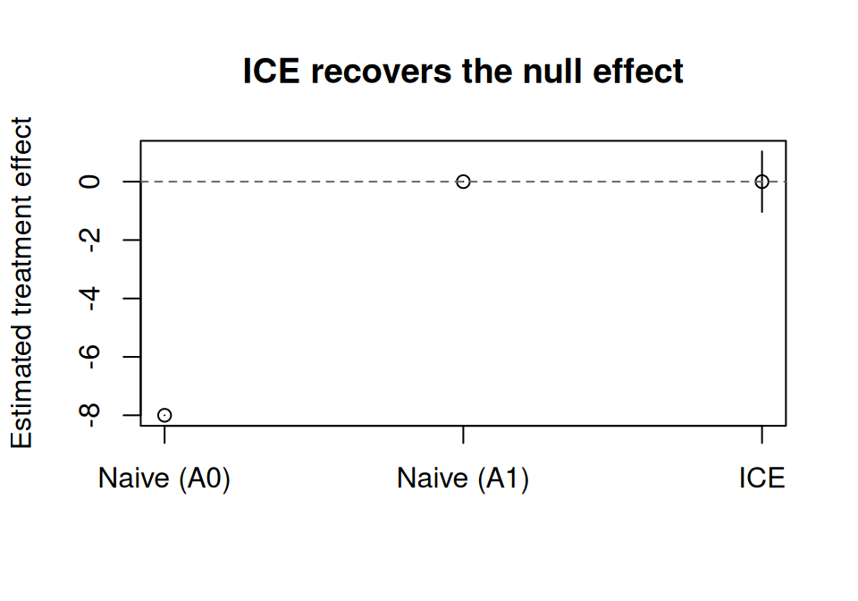

Point estimates and confidence intervals comparing naive regression to ICE g-computation. Naive estimates are biased away from zero while ICE correctly recovers ATE = 0.

Sandwich SE: stacked estimating equations

The default ci_method = "sandwich" uses the empirical sandwich estimator for stacked estimating equations (Zivich et al., 2024). This accounts for uncertainty from all K sequential outcome models, not just the final model.

Code

result$estimates[, c("intervention", "estimate", "se")]
#>    intervention estimate        se
#>          <char>    <num>     <num>
#> 1:       always       60 0.4000000
#> 2:        never       60 0.3464102

The standard errors are finite and positive, confirming that the sandwich variance estimator is working correctly even with a large sample.

Bootstrap SE

For robustness or when using flexible models (e.g., GAMs), bootstrap resamples individuals (all their time points together) and re-runs the full ICE procedure.

Code

result_boot <- contrast(
  fit,
  interventions = list(always = static(1), never = static(0)),
  reference = "never",
  type = "difference",
  ci_method = "bootstrap",
  n_boot = 20L
)
result_boot

Estimator: gcomp · Estimand: ATE · Contrast: difference · CI method: bootstrap · N: 3200

Intervention means
intervention	estimate	se	ci_lower	ci_upper
always	60	0.524	58.972	61.028
never	60	0.33	59.353	60.647

Contrasts
comparison	estimate	se	ci_lower	ci_upper
always vs never	-0.00000000000009947598	0.483	-0.947	0.947

The parallel and ncpus arguments enable parallel bootstrap replicates for larger datasets. Four backends are supported: "no" (sequential), "multicore" (Unix fork, default on most Linux/macOS setups), "snow" (cross-platform socket cluster, both via boot::boot()), and "future" (any active future::plan() — local multisession, remote plan(cluster, ...), or future.batchtools for HPC job arrays). "future" bypasses boot::boot() so the plan itself owns the scheduling; ncpus is ignored in that case.

Code

# boot::boot parallel (fork / socket)
result_par <- contrast(
  fit,
  interventions = list(always = static(1), never = static(0)),
  reference = "never",
  ci_method = "bootstrap",
  n_boot = 20L,
  parallel = "multicore",
  ncpus = 4L
)

# future backend (any future::plan())
library(future)
plan(multisession, workers = 4)
result_future <- contrast(
  fit,
  interventions = list(always = static(1), never = static(0)),
  reference = "never",
  ci_method = "bootstrap",
  n_boot = 500L,
  parallel = "future"
)

Comparing sandwich and bootstrap SEs

Code

se_df <- data.frame(
  method = c("Sandwich", "Bootstrap"),
  estimate = c(result$contrasts$estimate[1], result_boot$contrasts$estimate[1]),
  ci_lower = c(result$contrasts$ci_lower[1], result_boot$contrasts$ci_lower[1]),
  ci_upper = c(result$contrasts$ci_upper[1], result_boot$contrasts$ci_upper[1])
)
tinyplot(
  estimate ~ method,
  data = se_df,
  type = "pointrange",
  ymin = se_df$ci_lower,
  ymax = se_df$ci_upper,
  ylab = "ATE (always vs never)",
  xlab = "Inference method",
  main = "Sandwich vs bootstrap inference"
)
abline(h = 0, lty = 2, col = "grey40")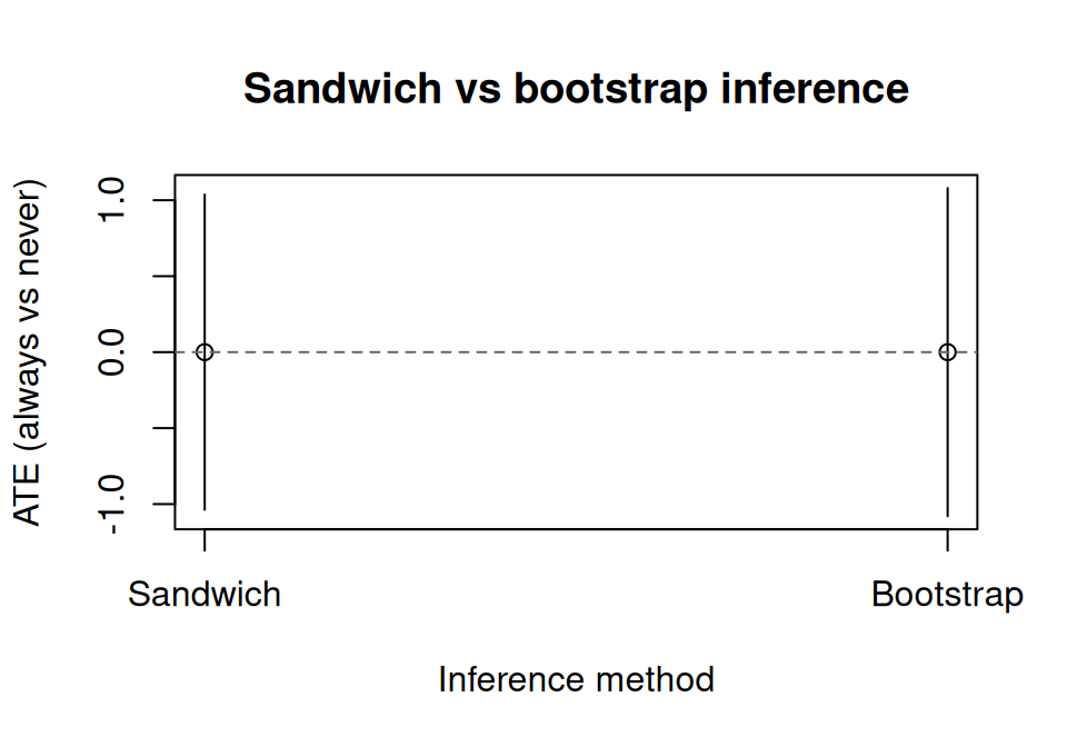

Point estimates and confidence intervals from sandwich and bootstrap inference for the ICE ATE estimate, showing close agreement.

Dynamic interventions

ICE supports dynamic treatment regimes where treatment depends on time-varying covariates. Here, individuals receive treatment only when L = 1 (the confounder is present):

Code

result_dyn <- contrast(
  fit,
  interventions = list(
    adaptive = dynamic(
      \(data, trt) ifelse(!is.na(data$L) & data$L > 0, 1L, 0L)
    ),
    always   = static(1),
    never    = static(0)
  ),
  reference = "never",
  ci_method = "sandwich"
)
result_dyn

Estimator: gcomp · Estimand: ATE · Contrast: difference · CI method: sandwich · N: 3200

Intervention means
intervention	estimate	se	ci_lower	ci_upper
adaptive	60	0.346	59.321	60.679
always	60	0.4	59.216	60.784
never	60	0.346	59.321	60.679

Contrasts
comparison	estimate	se	ci_lower	ci_upper
adaptive vs never	-0.00000000000006394885	0	-0	0
always vs never	-0.00000000000009947598	0.529	-1.037	1.037

Comparing multiple interventions

Code

est <- result_dyn$estimates
tinyplot(
  estimate ~ intervention,
  data = est,
  type = "pointrange",
  ymin = est$ci_lower,
  ymax = est$ci_upper,
  ylab = "E[Y^a]",
  xlab = "Intervention",
  main = "Marginal means under different interventions"
)
abline(h = 60, lty = 2, col = "grey40")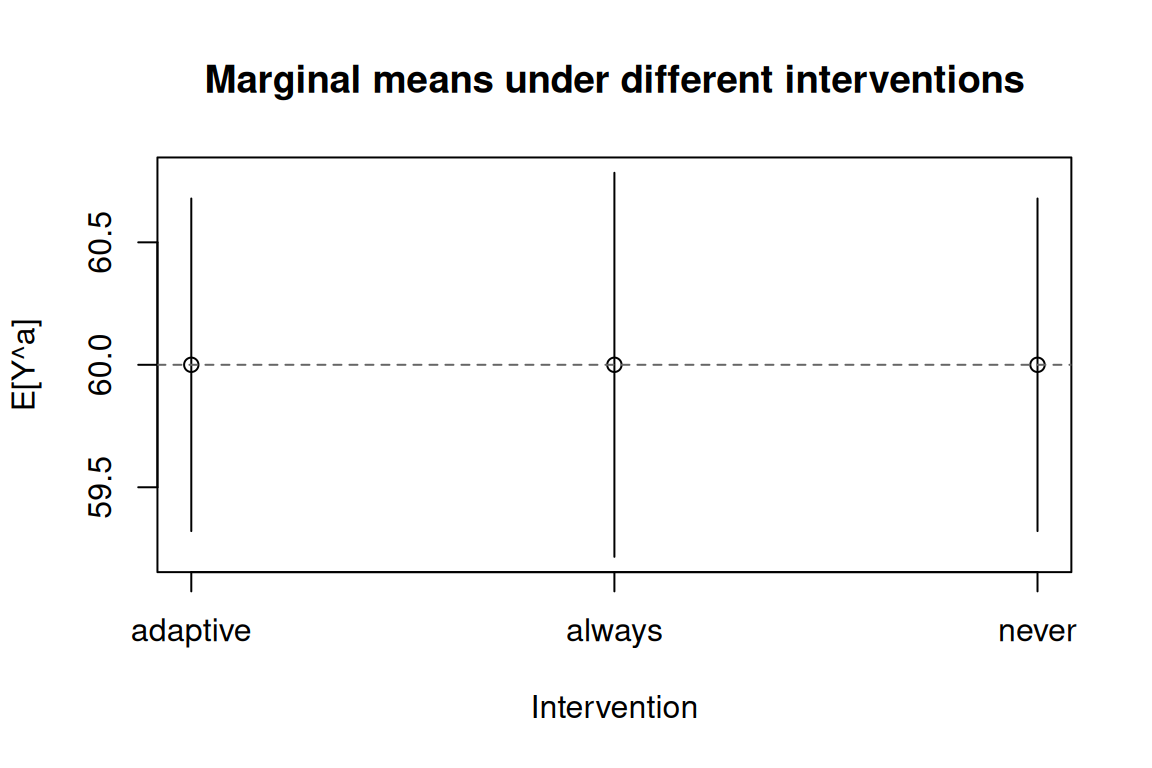

Forest plot of marginal means under three interventions: always treat, never treat, and adaptive (treat if L=1). All are close to 60 in this null-effect example.

All three interventions should return a marginal mean close to 60 (the structural truth for every joint regime in this null-effect DGP).

The `history` parameter

The history parameter controls the Markov order — how many lags of treatment and time-varying confounders enter each outcome model.

history = 1 (default): Include one lag of A and L (first-order Markov).
history = 2: Include two lags (A_{k-1}, A_{k-2}, L_{k-1}, L_{k-2}).
history = Inf: Include full treatment and confounder history up to each time point.

For this 2-time-point example, history = 1 and history = Inf are equivalent. With longer follow-up, higher-order histories capture longer-range dependencies but require more data per model.

Code

fit_inf <- causat(
  long,
  outcome = "Y",
  treatment = "A",
  confounders = ~ 1,
  confounders_tv = ~ L,
  id = "id",
  time = "time",
  history = Inf,
  model_fn = stats::glm
)

result_inf <- contrast(
  fit_inf,
  interventions = list(always = static(1), never = static(0)),
  reference = "never",
  ci_method = "sandwich"
)
result_inf

Estimator: gcomp · Estimand: ATE · Contrast: difference · CI method: sandwich · N: 3200

Intervention means
intervention	estimate	se	ci_lower	ci_upper
always	60	0.4	59.216	60.784
never	60	0.346	59.321	60.679

Contrasts
comparison	estimate	se	ci_lower	ci_upper
always vs never	-0.00000000000009947598	0.529	-1.037	1.037

Simulation: ICE with a non-null effect

To show ICE working with a known non-null effect, we simulate data with treatment-confounder feedback.

DGM. Two periods ($k = 0, 1$) with binary treatment $A_k \in \{0, 1\}$, binary time-varying confounder $L_k \in \{0, 1\}$, and continuous outcome $Y$. Treatment assignment at each period depends on the current confounder via a logistic model; the confounder at $k = 1$ is affected by prior treatment $A_0$ (treatment-confounder feedback). The structural equations are:

\[ \begin{aligned} L_0 &\sim \text{Bernoulli}(0.5), \\ A_0 \mid L_0 &\sim \text{Bernoulli}\bigl(\text{logit}^{-1}(-0.5 + 0.5 \, L_0)\bigr), \\ L_1 \mid A_0, L_0 &\sim \text{Bernoulli}\bigl(\text{logit}^{-1}(-0.5 + 0.8 \, A_0 + 0.3 \, L_0)\bigr), \\ A_1 \mid L_1 &\sim \text{Bernoulli}\bigl(\text{logit}^{-1}(-0.5 + 0.5 \, L_1)\bigr), \\ Y \mid A_0, A_1, L_1 &= 50 + 2.5 \, A_0 + 2.5 \, A_1 - 3 \, L_1 + \varepsilon, \quad \varepsilon \sim N(0, 25). \end{aligned} \]

The structural ATE of “always treat” vs “never treat” is not simply $2.5 + 2.5 = 5$, because $A_0$ affects $L_1$ (coefficient $0.8$), and $L_1$ enters the outcome with coefficient $-3$. Under “always treat”, $A_0 = 1$ increases $\mathbb{E}[L_1]$, and since $L_1$ has a negative effect on $Y$, this indirect path partially offsets the direct benefit:

\[ \text{ATE} = \underbrace{(2.5 + 2.5)}_{\text{direct}} - 3 \bigl(\mathbb{E}[L_1 \mid A_0\!=\!1] - \mathbb{E}[L_1 \mid A_0\!=\!0]\bigr) \approx 5 - 3 \times 0.196 \approx 4.41. \]

This is the same treatment-confounder feedback that makes naive regression biased.

Code

set.seed(42)
n <- 2000
sim_id <- rep(seq_len(n), each = 2)
sim_time <- rep(0:1, n)

L0 <- rbinom(n, 1, 0.5)
A0 <- rbinom(n, 1, plogis(-0.5 + 0.5 * L0))
L1 <- rbinom(n, 1, plogis(-0.5 + 0.8 * A0 + 0.3 * L0))
A1 <- rbinom(n, 1, plogis(-0.5 + 0.5 * L1))
Y <- 50 + 2.5 * A0 + 2.5 * A1 - 3 * L1 + rnorm(n, 0, 5)

sim_long <- data.frame(
  id = sim_id,
  time = sim_time,
  A = c(rbind(A0, A1)),
  L = c(rbind(L0, L1)),
  Y = c(rbind(NA_real_, Y))
)

fit_sim <- causat(
  sim_long,
  outcome = "Y",
  treatment = "A",
  confounders = ~ 1,
  confounders_tv = ~ L,
  id = "id",
  time = "time",
  model_fn = stats::glm
)

res_sim <- contrast(
  fit_sim,
  interventions = list(always = static(1), never = static(0)),
  reference = "never",
  ci_method = "sandwich"
)
res_sim

Estimator: gcomp · Estimand: ATE · Contrast: difference · CI method: sandwich · N: 2000

Intervention means
intervention	estimate	se	ci_lower	ci_upper
always	53.134	0.227	52.69	53.579
never	48.832	0.187	48.465	49.199

Contrasts
comparison	estimate	se	ci_lower	ci_upper
always vs never	4.303	0.336	3.644	4.961

The estimated ATE should be close to the true value of $\approx 4.41$.

Binary outcome

ICE also handles binary outcomes. The first outcome model uses binomial (actual 0/1 response), while subsequent pseudo-outcome models use quasibinomial (fractional logistic for predicted probabilities in [0, 1]).

DGM. This reuses the non-null simulation above (same SEM) with the continuous outcome binarised at $Y > 50$:

\[ \begin{aligned} Y^* &= 50 + 2.5 \, A_0 + 2.5 \, A_1 - 3 \, L_1 + \varepsilon, \quad \varepsilon \sim N(0, 25), \\ Y &= \mathbf{1}(Y^* > 50). \end{aligned} \]

The resulting binary outcome does not have a clean closed-form ATE on the risk-difference scale, but the direction is positive (“always treat” increases $P(Y = 1)$ relative to “never treat”) because both treatment coefficients are positive in the latent linear predictor.

Code

sim_long_bin <- sim_long
sim_long_bin$Y[!is.na(sim_long_bin$Y)] <-
  as.integer(sim_long_bin$Y[!is.na(sim_long_bin$Y)] > 50)

fit_bin <- causat(
  sim_long_bin,
  outcome = "Y",
  treatment = "A",
  confounders = ~ 1,
  confounders_tv = ~ L,
  family = "binomial",
  id = "id",
  time = "time",
  model_fn = stats::glm
)

res_bin <- contrast(
  fit_bin,
  interventions = list(always = static(1), never = static(0)),
  reference = "never",
  type = "difference",
  ci_method = "sandwich"
)
res_bin

Estimator: gcomp · Estimand: ATE · Contrast: difference · CI method: sandwich · N: 2000

Intervention means
intervention	estimate	se	ci_lower	ci_upper
always	0.728	0.018	0.693	0.764
never	0.415	0.018	0.381	0.449

Contrasts
comparison	estimate	se	ci_lower	ci_upper
always vs never	0.313	0.029	0.256	0.371

Risk ratio for binary longitudinal outcomes

Code

res_rr <- contrast(
  fit_bin,
  interventions = list(always = static(1), never = static(0)),
  reference = "never",
  type = "ratio",
  ci_method = "sandwich"
)
res_rr

Estimator: gcomp · Estimand: ATE · Contrast: ratio · CI method: sandwich · N: 2000

Intervention means
intervention	estimate	se	ci_lower	ci_upper
always	0.728	0.018	0.693	0.764
never	0.415	0.018	0.381	0.449

Contrasts
comparison	estimate	se	ci_lower	ci_upper
always vs never	1.754	0.098	1.572	1.958

Three or more time periods

The examples above use 2 time points for simplicity, but ICE scales to any number of periods. Here we simulate 4-period data with a binary treatment and binary outcome. The backward recursion fits 4 sequential models.

DGM. Four periods ($k = 1, \dots, 4$) with binary treatment $A_k$, continuous time-varying confounder $L_k$, continuous baseline confounder $L_0$, and binary outcome $Y$ measured at $k = 4$. The confounder evolves with treatment feedback: at each step, $L_k$ depends on $L_{k-1}$ plus noise, and after observing $A_k$ the next confounder shifts by $0.3 \, A_k$. The structural equations are:

\[ \begin{aligned} L_0 &\sim N(0, 1), \\ L_k \mid L_{k-1}, A_{k-1} &= L_{k-1} + 0.3 \, A_{k-1} + \eta_k, \quad \eta_k \sim N(0, 0.25), \\ A_k \mid L_k &\sim \text{Bernoulli}\bigl(\text{logit}^{-1}(-0.3 + 0.4 \, L_k)\bigr), \\ Y \mid A_1, \dots, A_4, L_0 &\sim \text{Bernoulli}\bigl(\text{logit}^{-1}(-1.5 + 0.4 \, \textstyle\sum_{k=1}^{4} A_k + 0.3 \, L_0)\bigr). \end{aligned} \]

The outcome depends on cumulative treatment exposure $\sum_k A_k$ and the baseline confounder $L_0$. Under “always treat” ($\sum A_k = 4$) the log-odds shift by $0.4 \times 4 = 1.6$ relative to “never treat” ($\sum A_k = 0$), so the risk difference on the probability scale is positive but does not have a simple closed form (it depends on the marginal distribution of $L_0$).

Code

set.seed(99)
n_id <- 600
K <- 4

ids <- rep(seq_len(n_id), each = K)
times <- rep(seq_len(K), n_id)

L0 <- rep(rnorm(n_id), each = K)
sim_4p <- data.frame(id = ids, time = times, L0 = L0)

sim_4p$L <- NA_real_
sim_4p$A <- NA_integer_
for (i in seq_len(n_id)) {
  rows <- which(sim_4p$id == i)
  l_prev <- sim_4p$L0[rows[1]]
  for (k in seq_along(rows)) {
    sim_4p$L[rows[k]] <- l_prev + rnorm(1, 0, 0.5)
    sim_4p$A[rows[k]] <- rbinom(1, 1, plogis(-0.3 + 0.4 * sim_4p$L[rows[k]]))
    l_prev <- sim_4p$L[rows[k]] + 0.3 * sim_4p$A[rows[k]]
  }
}

sim_4p$Y <- NA_real_
for (i in seq_len(n_id)) {
  rows <- which(sim_4p$id == i)
  cum_a <- sum(sim_4p$A[rows])
  sim_4p$Y[rows[K]] <- rbinom(
    1, 1,
    plogis(-1.5 + 0.4 * cum_a + 0.3 * sim_4p$L0[rows[1]])
  )
}

fit_4p <- causat(
  sim_4p,
  outcome = "Y",
  treatment = "A",
  confounders = ~ L0,
  confounders_tv = ~ L,
  family = "binomial",
  id = "id",
  time = "time",
  model_fn = stats::glm
)

res_4p <- contrast(
  fit_4p,
  interventions = list(always = static(1), never = static(0)),
  reference = "never",
  type = "difference",
  ci_method = "sandwich"
)
res_4p

Estimator: gcomp · Estimand: ATE · Contrast: difference · CI method: sandwich · N: 600

Intervention means
intervention	estimate	se	ci_lower	ci_upper
always	0.528	0.052	0.426	0.63
never	0.166	0.029	0.109	0.222

Contrasts
comparison	estimate	se	ci_lower	ci_upper
always vs never	0.362	0.073	0.219	0.506

Code

plot(res_4p)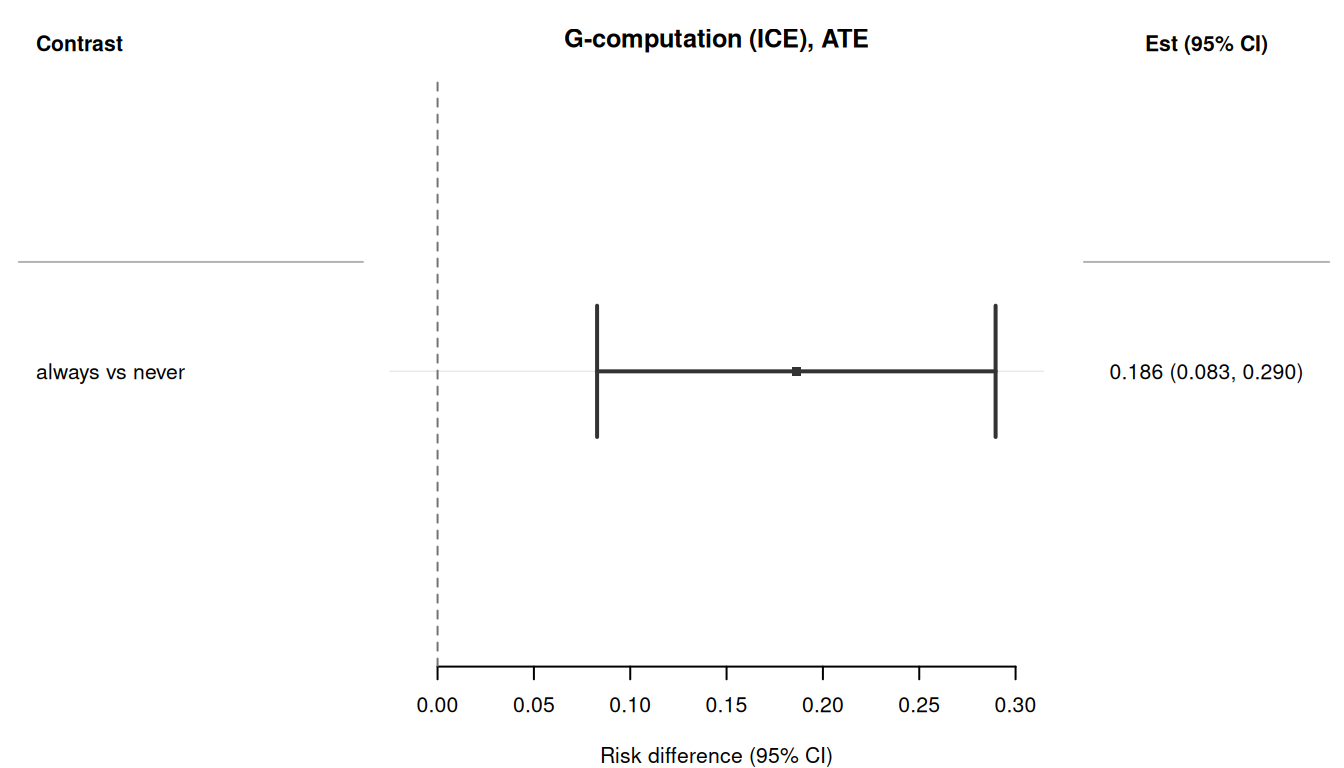

Forest plot showing the risk difference between always-treat and never-treat over 4 periods.

Code

tt(tidy(res_4p), digits = 3)

term	estimate	std.error	type	conf.low	conf.high
always vs never	0.362	0.0733	contrast	0.219	0.506

The ICE sandwich variance correctly propagates uncertainty through all 4 sequential models via the stacked estimating equations cascade.

Continuous treatment with modified treatment policies

ICE also supports continuous time-varying treatments combined with the modified-treatment-policy (MTP) interventions: shift(), scale_by(), and threshold(). The intervention is applied to the current-time treatment at each backward step; ice_apply_intervention_long() explicitly does not recompute the lag columns from the intervened values (this would double-count a non-static intervention — see CLAUDE.md for the structural reason).

DGM. Two periods ($k = 0, 1$) with continuous treatment $A_k \in \mathbb{R}$, continuous confounder $L_k$, and continuous outcome $Y$. Treatment-confounder feedback is present: $A_0$ affects $L_1$ (coefficient $0.5$), and $L_1$ affects $A_1$ (coefficient $0.5$). The structural equations are:

\[ \begin{aligned} L_0 &\sim N(0, 1), \\ A_0 &= 1 + 0.4 \, L_0 + \eta_0, \quad \eta_0 \sim N(0, 1), \\ L_1 &= 0.3 \, L_0 + 0.5 \, A_0 + \eta_1, \quad \eta_1 \sim N(0, 1), \\ A_1 &= 1 + 0.5 \, L_1 + \eta_2, \quad \eta_2 \sim N(0, 1), \\ Y &= 2 + 1.5 \, A_0 + 2 \, A_1 + 0.5 \, L_0 - 0.3 \, L_1 + \varepsilon, \quad \varepsilon \sim N(0, 1). \end{aligned} \]

For a shift(-1) MTP (reduce each $A_k$ by 1 at each period), the structural causal effect on $Y$ relative to the natural course accounts for both direct and indirect paths. Shifting $A_0$ by $-1$ also shifts $L_1$ by $-0.5$ (coefficient $0.5$ in the $L_1$ equation), which in turn shifts the natural value of $A_1$ by $-0.25$ (coefficient $0.5$ in the $A_1$ equation). The shifted $A_1$ is then reduced by a further $-1$ by the MTP. The total effect on $Y$ is:

\[ 1.5 \times (-1) + 2 \times (-1.25) + (-0.3) \times (-0.5) = -1.5 - 2.5 + 0.15 = -3.85. \]

Code

set.seed(101)
n <- 800
sim_id <- rep(seq_len(n), each = 2)
sim_time <- rep(0:1, n)

L0 <- rnorm(n)
A0 <- 1 + 0.4 * L0 + rnorm(n)
L1 <- 0.3 * L0 + 0.5 * A0 + rnorm(n)
A1 <- 1 + 0.5 * L1 + rnorm(n)
Y <- 2 + 1.5 * A0 + 2 * A1 + 0.5 * L0 - 0.3 * L1 + rnorm(n)

cont_long <- data.frame(
  id = sim_id,
  time = sim_time,
  A = c(rbind(A0, A1)),
  L = c(rbind(L0, L1)),
  Y = c(rbind(NA_real_, Y))
)

fit_cont <- causat(
  cont_long,
  outcome = "Y",
  treatment = "A",
  confounders = ~ 1,
  confounders_tv = ~ L,
  id = "id",
  time = "time",
  model_fn = stats::glm
)

res_mtp <- contrast(
  fit_cont,
  interventions = list(
    observed = NULL,
    shift_m1 = shift(-1),
    halved   = scale_by(0.5),
    capped   = threshold(0, 1)
  ),
  reference = "observed",
  type = "difference",
  ci_method = "sandwich"
)
res_mtp

Estimator: gcomp · Estimand: ATE · Contrast: difference · CI method: sandwich · N: 800

Intervention means
intervention	estimate	se	ci_lower	ci_upper
observed	5.904	0.117	5.675	6.134
shift_m1	2.061	0.147	1.773	2.349
halved	3.799	0.075	3.652	3.946
capped	4.326	0.059	4.21	4.443

Contrasts
comparison	estimate	se	ci_lower	ci_upper
shift_m1 vs observed	-3.844	0.086	-4.013	-3.674
halved vs observed	-2.105	0.066	-2.235	-1.976
capped vs observed	-1.578	0.084	-1.743	-1.414

Structural truth for shift(-1) is $-3.85$ (see derivation above). The shift_m1 estimate should be close to this value.

Flexible treatment terms (`treatment_form`)

By default the treatment enters every per-step outcome model as a bare numeric main effect. For a binary treatment that is saturated, but for an ordered / ordinal dose a single linear slope can misspecify a non-monotone or kinked counterfactual dose-response. treatment_form lets the dose enter the per-step model via a transformed term — ~ factor(A) or ~ splines::ns(A, df) — while the intervention still sets the numeric dose column. Lag terms expand automatically (factor(A) → factor(lag1_A)).

DGM. Two periods, a 3-level dose $A_k \in \{0, 1, 2\}$ confounded by an exogenous covariate, and a deliberately non-monotone level effect $f(0) = 0,\ f(1) = 3,\ f(2) = 1$ with $Y = 1 + f(A_0) + f(A_1) + 0.5\,L_0 + \varepsilon$. Because the covariate does not depend on past treatment, the contrast $E[Y^{\text{static}(1)}] - E[Y^{\text{static}(0)}] = 2\,(f(1) - f(0)) = 6$ exactly.

Code

set.seed(1)
n <- 4000
f_lvl <- c(0, 3, 1) # f(0), f(1), f(2): non-monotone
L0 <- rnorm(n)
mk_period <- function() {
  Lt <- 0.5 * L0 + rnorm(n)
  At <- pmin(2L, rpois(n, exp(-0.3 + 0.5 * Lt)))
  list(L = Lt, A = At)
}
p0 <- mk_period()
p1 <- mk_period()
Yv <- 1 + f_lvl[p0$A + 1] + f_lvl[p1$A + 1] + 0.5 * L0 + rnorm(n)

dose_long <- data.frame(
  id = rep(seq_len(n), each = 2),
  time = rep(0:1, n),
  A = c(rbind(p0$A, p1$A)),
  L = c(rbind(p0$L, p1$L)),
  Y = c(rbind(NA_real_, Yv))
)

fit_args <- list(
  data = dose_long, outcome = "Y", treatment = "A",
  confounders = ~1, confounders_tv = ~L,
  id = "id", time = "time", estimator = "gcomp", model_fn = stats::glm
)
fit_bare <- do.call(causat, fit_args)
fit_factor <- do.call(causat, c(fit_args, list(treatment_form = ~ factor(A))))

ivs <- list(a1 = static(1), a0 = static(0))
diff_of <- function(fit) {
  r <- contrast(fit, interventions = ivs, type = "difference")
  with(r$estimates, estimate[intervention == "a1"] - estimate[intervention == "a0"])
}
dose_compare <- data.frame(
  model = c("bare numeric A", "factor(A)"),
  contrast = c(diff_of(fit_bare), diff_of(fit_factor)),
  truth = 6
)
tinytable::tt(dose_compare, digits = 3)

model	contrast	truth
bare numeric A	1.83	6
factor(A)	6	6

The bare-numeric model fits one slope through the non-monotone response and is far from the truth of 6; ~ factor(A) gives each dose level its own coefficient and recovers it to sampling error. The flexible term is longitudinal g-computation only and also powers natural-history dose policies (see the Natural-history MTPs vignette). Under factor(A) an intervention must stay within the observed dose levels; splines::ns(A, df) extrapolates smoothly.

Longitudinal IPW (sequential density-ratio weights)

ICE g-computation models the outcome at each period and iterates backward. The IPW analogue models the treatment density at each period and accumulates a per-id density-ratio weight, then fits a weighted final-period MSM. Both target the same counterfactual mean $E[Y^d]$; agreement between them is the methodological-triangulation test causatr is built around.

The mathematical structure is the same chain rule we used for multivariate IPW (Phase 8) but indexed by time rather than treatment component. For an intervention $d$ applied at every period $k = 0, 1, \ldots, K$:

\[ W_i = \prod_{k=0}^{K} \frac{f_k\bigl(d(A_{k,i}, L_{k,i}) \mid \bar A_{k-1,i}^{\mathrm{obs}}, \bar L_{k,i}\bigr) \cdot \lvert \mathrm{Jac}\,d^{-1} \rvert}{f_k\bigl(A_{k,i} \mid \bar A_{k-1,i}^{\mathrm{obs}}, \bar L_{k,i}\bigr)}. \]

Both numerator and denominator condition on observed upstream treatments — the sequential-MTP semantics of Robins, Hernán, Brumback (2000) and Díaz et al. (2023). The MSM is intercept-only Hájek on the final-period rows, weighted by the per-id cumulative product; the (sole) coefficient is $E[Y^d]$.

Code

fit_ipw_long <- causat(
  cont_long,
  outcome     = "Y",
  treatment   = "A",
  confounders = ~ 1,
  confounders_tv = ~ L,
  id          = "id",
  time        = "time",
  estimator   = "ipw",
  model_fn = stats::glm,
  propensity_model_fn = stats::glm
)

res_ipw_long <- contrast(
  fit_ipw_long,
  interventions = list(observed = NULL, shift_m1 = shift(-1)),
  reference     = "observed",
  type          = "difference",
  ci_method     = "sandwich"
)
res_ipw_long

Estimator: ipw · Estimand: ATE · Contrast: difference · CI method: sandwich · N: 800

Intervention means
intervention	estimate	se	ci_lower	ci_upper
observed	5.904	0.117	5.675	6.134
shift_m1	2.341	0.254	1.842	2.839

Contrasts
comparison	estimate	se	ci_lower	ci_upper
shift_m1 vs observed	-3.564	0.234	-4.022	-3.105

ICE g-comp and longitudinal IPW estimate the same target parameter, so on a correctly-specified linear-Gaussian DGP they should agree on the point estimate up to Monte Carlo error. Sandwich SEs differ — IPW typically has heavier variance than g-computation when the outcome model is correct, so the IPW SE is usually larger.

Code

res_mtp$contrasts
#>              comparison  estimate         se  ci_lower  ci_upper
#>                  <char>     <num>      <num>     <num>     <num>
#> 1: shift_m1 vs observed -3.843574 0.08631052 -4.012739 -3.674408
#> 2:   halved vs observed -2.105375 0.06595945 -2.234654 -1.976097
#> 3:   capped vs observed -1.578207 0.08385391 -1.742558 -1.413857
res_ipw_long$contrasts
#>              comparison  estimate        se  ci_lower  ci_upper
#>                  <char>     <num>     <num>     <num>     <num>
#> 1: shift_m1 vs observed -3.563666 0.2337656 -4.021838 -3.105494

Supported interventions. static() / shift() / scale_by() / dynamic() are dispatched per period through the same family-aware gates as point IPW (check_intervention_family_compat()). Natural course (NULL) collapses every per-period weight to 1 and recovers the observed marginal mean. ipsi() is supported for univariate binary treatment via a per-period Kennedy product (see below).

Bootstrap. ci_method = "bootstrap" resamples individuals (every person-period row of a sampled id travels together). Cloning ids that are sampled multiple times mirrors the ICE bootstrap convention so within-person dependence is preserved.

Code

res_ipw_boot <- contrast(
  fit_ipw_long,
  interventions = list(observed = NULL, shift_m1 = shift(-1)),
  reference     = "observed",
  type          = "difference",
  ci_method     = "bootstrap",
  n_boot        = 100
)
res_ipw_boot$contrasts
#>              comparison  estimate        se  ci_lower  ci_upper
#>                  <char>     <num>     <num>     <num>     <num>
#> 1: shift_m1 vs observed -3.563666 0.2346474 -4.023566 -3.103765

Sequential positivity warning. When any per-period weight has a heavy tail (max > 100 by default) the engine emits a causatr_longitudinal_seq_positivity warning naming the offending period(s) and their per-period max weight. The cumulative product loses period attribution, so this per-period diagnostic is the primary way to identify which time step is the bottleneck.

Stabilized weights

stabilize = "marginal" swaps each period’s numerator density for a marginal model $g_k(A_k \mid \bar A_{k-1}, V)$ that drops the time-varying confounder $L_k$ (and optionally adds a user-supplied baseline conditioning set $V$ via numerator = ~ V). The denominator stays at the full-$L$ density. Per-period weight becomes $g_k(d(A_k) \mid \bar A_{k-1}, V) \cdot \lvert \mathrm{Jac} \rvert / f_k(A_k \mid \bar A_{k-1}, \bar L_k)$, which dampens the multiplicative $L$-dependence across $K$ factors and typically reduces the cumulative product’s variance.

Code

fit_ipw_long_stab <- causat(
  cont_long,
  outcome     = "Y",
  treatment   = "A",
  confounders = ~ 1,
  confounders_tv = ~ L,
  id          = "id",
  time        = "time",
  estimator   = "ipw",
  stabilize   = "marginal",
  model_fn = stats::glm,
  propensity_model_fn = stats::glm
)

contrast(
  fit_ipw_long_stab,
  interventions = list(observed = NULL, shift_m1 = shift(-1)),
  reference     = "observed",
  type          = "difference",
  ci_method     = "sandwich"
)

Estimator: ipw · Estimand: ATE · Contrast: difference · CI method: sandwich · N: 800

Intervention means
intervention	estimate	se	ci_lower	ci_upper
observed	5.904	0.08	5.747	6.061
shift_m1	2.805	0.175	2.462	3.147

Contrasts
comparison	estimate	se	ci_lower	ci_upper
shift_m1 vs observed	-3.1	0.173	-3.439	-2.76

By default the per-period numerator drops every confounder and conditions only on prior treatment lags. A custom numerator = formula adds baseline-only covariates on top of the lags, which typically gives the most stable contrast estimate when the structural treatment generation depends on baseline characteristics.

Sandwich variance treats the numerator parameters as fixed (same nuisance-fixed convention as Phase 8e for multivariate IPW); bootstrap refits both numerator and denominator per replicate and captures the full uncertainty.

Effect modification (baseline modifier)

When confounders = includes an A:modifier interaction term, the per-period propensity formulas automatically strip the treatment-touching interaction (the modifier main effect is kept), and the final-period MSM expands from Y ~ 1 to Y ~ 1 + modifier so predict() returns stratum-specific counterfactual means.

Code

fit_em <- causat(
  long_data,
  outcome     = "Y",
  treatment   = "A",
  confounders = ~ baseline + sex + A:sex,
  confounders_tv = ~ L,
  id          = "id",
  time        = "time",
  estimator   = "ipw",
  model_fn = stats::glm,
  propensity_model_fn = stats::glm
)
contrast(
  fit_em,
  interventions = list(a = static(1), z = static(0)),
  reference     = "z",
  by            = "sex"
)

Known limitation (Robins 2000). Under longitudinal IPW, the modifier MUST be a baseline covariate. A time-varying modifier in an MSM conditions on a post-treatment variable, which biases the estimand via mediator and collider paths. causatr does not enforce baseline-ness at runtime (time-varying status isn’t inferable from data); the constraint is documented only. The scientifically correct tool for time-varying effect modification is a structural nested model — use estimator = "snm" with id = and time = (see vignette("snm")).

Baseline effect modification also composes with multivariate longitudinal treatment: each per-period × per-component propensity strips its own A_k:modifier interactions (keeping the modifier as a confounder main effect), and the single final-period MSM still expands to Y ~ 1 + modifier. Specify the interaction once per component, e.g. confounders = ~ baseline + sex + A1:sex + A2:sex with treatment = c("A1", "A2").

Incremental propensity-score interventions (IPSI)

For binary time-varying treatment, ipsi(delta) shifts the treatment odds at every period by a factor $\delta$ rather than fixing a counterfactual value. Kennedy’s (2019) closed-form weight extends to a per-period product:

\[ W_i = \prod_{t=1}^{T} \frac{\delta \, A_{t,i} + (1 - A_{t,i})} {\delta \, p_{t,i} + (1 - p_{t,i})}, \qquad p_{t,i} = P(A_t = 1 \mid \bar A_{t-1}, \bar L_t). \]

$\delta = 1$ recovers the natural course (every factor is 1); $\delta > 1$ nudges everyone toward treatment, $\delta < 1$ away from it. Because each denominator stays in $[\min(1, \delta), \max(1, \delta)]$, the per-period weights are bounded by construction — IPSI is a stable alternative to deterministic “always treat” contrasts when positivity is borderline.

Code

set.seed(204)
n_ip <- 800
ip_id <- rep(seq_len(n_ip), each = 2)
ip_time <- rep(0:1, n_ip)
L0_ip <- rnorm(n_ip)
A0_ip <- rbinom(n_ip, 1, plogis(0.5 * L0_ip))
L1_ip <- 0.5 * L0_ip + 0.4 * A0_ip + rnorm(n_ip)
A1_ip <- rbinom(n_ip, 1, plogis(0.3 * L1_ip + 0.2 * A0_ip))
Y_ip <- 10 + 2 * (A0_ip + A1_ip) + L0_ip + L1_ip + rnorm(n_ip)
ipsi_long <- data.frame(
  id = ip_id,
  time = ip_time,
  A = as.vector(rbind(A0_ip, A1_ip)),
  L = as.vector(rbind(L0_ip, L1_ip)),
  L0 = rep(L0_ip, each = 2),
  Y = as.vector(rbind(rep(NA_real_, n_ip), Y_ip))
)

fit_ipsi_long <- causat(
  ipsi_long,
  outcome     = "Y",
  treatment   = "A",
  confounders = ~ L0,
  confounders_tv = ~ L,
  id          = "id",
  time        = "time",
  estimator   = "ipw"
)
#> Warning: `model_fn` not specified; defaulting to `stats::glm`.
#> ℹ Set `model_fn` explicitly (e.g. `model_fn = stats::glm` or `model_fn = mgcv::gam`).
#> Warning: `propensity_model_fn` not specified; defaulting to `stats::glm`.
#> ℹ Set `propensity_model_fn` explicitly if you need a different fitter (e.g. `mgcv::gam`).
#> Warning: Treatment model has aliased (collinear) coefficient(s): L0. Dropping from the sandwich variance computation.
#> Treatment model has aliased (collinear) coefficient(s): L0. Dropping from the sandwich variance computation.

res_ipsi <- contrast(
  fit_ipsi_long,
  interventions = list(
    down = ipsi(0.5),
    observed = ipsi(1),
    up = ipsi(2)
  ),
  ci_method = "sandwich"
)
tt(tidy(res_ipsi), digits = 3)

term	estimate	std.error	type	conf.low	conf.high
observed vs down	0.734	0.0248	contrast	0.685	0.782
up vs down	1.462	0.047	contrast	1.37	1.554

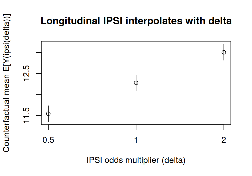
The three means interpolate monotonically: lowering the treatment odds ($\delta = 0.5$) pulls the counterfactual mean below the natural course ($\delta = 1$), raising them ($\delta = 2$) pushes it up.

Code

ipsi_df <- res_ipsi$estimates
ipsi_df$delta <- c(0.5, 1, 2)[match(
  ipsi_df$intervention,
  c("down", "observed", "up")
)]
ipsi_df <- ipsi_df[order(ipsi_df$delta), ]
tinyplot(
  estimate ~ factor(delta),
  data = ipsi_df,
  type = "pointrange",
  ymin = ipsi_df$ci_lower,
  ymax = ipsi_df$ci_upper,
  ylab = "Counterfactual mean E[Y(ipsi(delta))]",
  xlab = "IPSI odds multiplier (delta)",
  main = "Longitudinal IPSI interpolates with delta"
)

Point estimates and confidence intervals for IPSI counterfactual means at delta = 0.5, 1, and 2. The means increase monotonically with delta.

ipsi() under longitudinal IPW is univariate binary only. Multivariate IPSI (treatment = c("A1", "A2") with an ipsi() component) and ipsi() combined with stabilize = "marginal" are rejected with classed errors (causatr_longitudinal_ipsi_multivariate, causatr_longitudinal_ipsi_stabilize). Longitudinal AIPW does not support IPSI — use estimator = "ipw".

Weight truncation

With $T$ time periods, the cumulative product $\prod_{t=1}^{T} w_t$ of per-period density ratios can develop heavy tails. The trim argument on contrast() winsorizes density ratios at a given quantile before the cumulative product (Cole & Hernán 2008). trim = 0.999 clips each per-period ratio at its 99.9th percentile — the default in lmtp.

Code

res_ipw_trim <- contrast(
  fit_ipw_long,
  interventions = list(shift_m1 = shift(-1), observed = NULL),
  reference     = "observed",
  type          = "difference",
  ci_method     = "sandwich",
  trim          = 0.999
)
res_ipw_trim

Estimator: ipw · Estimand: ATE · Contrast: difference · CI method: sandwich · N: 800

Intervention means
intervention	estimate	se	ci_lower	ci_upper
shift_m1	2.402	0.236	1.94	2.864
observed	5.904	0.117	5.675	6.134

Contrasts
comparison	estimate	se	ci_lower	ci_upper
shift_m1 vs observed	-3.502	0.213	-3.919	-3.085

The default trim = 1 applies no truncation. With stabilize = "marginal", stabilization and truncation compose: stabilized per-period ratios are truncated at the quantile threshold before the cumulative product.

Multivariate time-varying treatment

When multiple treatments vary over time (e.g. two drugs dosed jointly), pass a character vector to treatment = and supply each intervention as a named sub-list. Lag columns are built per-component by prepare_data().

DGM. Two periods ($k = 0, 1$) with two binary treatments $A_{1,k}, A_{2,k} \in \{0, 1\}$, a continuous confounder $L_k$, and continuous outcome $Y$. Both treatments at $k = 0$ feed into the confounder $L_1$, creating treatment-confounder feedback. The structural equations are:

\[ \begin{aligned} L_0 &\sim N(0, 1), \\ A_{1,0} \mid L_0 &\sim \text{Bernoulli}\bigl(\text{logit}^{-1}(0.3 \, L_0)\bigr), \\ A_{2,0} \mid L_0 &\sim \text{Bernoulli}\bigl(\text{logit}^{-1}(0.1 \, L_0)\bigr), \\ L_1 &= 0.3 \, L_0 + 0.4 \, A_{1,0} + 0.2 \, A_{2,0} + \eta, \quad \eta \sim N(0, 1), \\ A_{1,1} \mid L_1 &\sim \text{Bernoulli}\bigl(\text{logit}^{-1}(0.3 \, L_1)\bigr), \\ A_{2,1} \mid L_1 &\sim \text{Bernoulli}\bigl(\text{logit}^{-1}(0.1 \, L_1)\bigr), \\ Y &= 2 + 1.5 \, A_{1,0} + 1.5 \, A_{1,1} + 0.8 \, A_{2,0} + 0.8 \, A_{2,1} + 0.5 \, L_1 + \varepsilon, \quad \varepsilon \sim N(0, 1). \end{aligned} \]

The outcome is linear in both treatments at both periods. The structural ATE of “both on” vs “both off” includes the indirect path through $L_1$: setting $A_{1,0} = A_{2,0} = 1$ shifts $\mathbb{E}[L_1]$ by $0.4 + 0.2 = 0.6$ relative to “both off”, and $L_1$ enters $Y$ with coefficient $0.5$, adding $0.3$ to the direct sum $2 \times (1.5 + 0.8) = 4.6$:

\[ \text{ATE} = \underbrace{4.6}_{\text{direct}} + \underbrace{0.5 \times 0.6}_{\text{indirect via } L_1} = 4.9. \]

Code

set.seed(202)
n <- 600
sim_id <- rep(seq_len(n), each = 2)
sim_time <- rep(0:1, n)
L0 <- rnorm(n)
A10 <- rbinom(n, 1, plogis(0.3 * L0))
A20 <- rbinom(n, 1, plogis(0.1 * L0))
L1 <- 0.3 * L0 + 0.4 * A10 + 0.2 * A20 + rnorm(n)
A11 <- rbinom(n, 1, plogis(0.3 * L1))
A21 <- rbinom(n, 1, plogis(0.1 * L1))
Y <- 2 + 1.5 * A10 + 1.5 * A11 + 0.8 * A20 + 0.8 * A21 + 0.5 * L1 + rnorm(n)

mv_long <- data.frame(
  id = sim_id,
  time = sim_time,
  A1 = c(rbind(A10, A11)),
  A2 = c(rbind(A20, A21)),
  L = c(rbind(L0, L1)),
  Y = c(rbind(NA_real_, Y))
)

fit_mv_long <- causat(
  mv_long,
  outcome = "Y",
  treatment = c("A1", "A2"),
  confounders = ~ 1,
  confounders_tv = ~ L,
  id = "id",
  time = "time",
  model_fn = stats::glm
)

res_mv_long <- contrast(
  fit_mv_long,
  interventions = list(
    both_on  = list(A1 = static(1), A2 = static(1)),
    both_off = list(A1 = static(0), A2 = static(0))
  ),
  reference = "both_off",
  type = "difference"
)
res_mv_long

Estimator: gcomp · Estimand: ATE · Contrast: difference · CI method: sandwich · N: 600

Intervention means
intervention	estimate	se	ci_lower	ci_upper
both_on	6.914	0.095	6.728	7.1
both_off	1.967	0.098	1.774	2.16

Contrasts
comparison	estimate	se	ci_lower	ci_upper
both_on vs both_off	4.947	0.17	4.613	5.281

Structural truth: both_on − both_off = 4.9 (direct effects $4.6$ plus indirect $0.3$ via $L_1$).

Stabilization with multivariate treatments

stabilize = "marginal" composes with multivariate longitudinal IPW. The marginal numerator factorises over both axes: per period and per component. Each component’s numerator drops the time-varying confounders $L$ but keeps the treatment lags and the within-period prior components $A_{1,\dots,k-1}$, mirroring the denominator chain rule:

\[ g(\bar{A}_1, \bar{A}_2 \mid V) = \prod_t \prod_k g_{t,k}\bigl(A_{t,k} \mid A_{t,1:k-1}, \bar{A}_{t-1}, V\bigr). \]

Under static interventions on binary treatments the stabilized and unstabilized estimates coincide exactly — the indicator pins every conditioning variable to the target, so numerator and denominator densities cancel on the surviving rows:

Code

fit_mv_long_stab <- causat(
  mv_long,
  outcome = "Y",
  treatment = c("A1", "A2"),
  confounders = ~ 1,
  confounders_tv = ~ L,
  id = "id",
  time = "time",
  model_fn = stats::glm,
  stabilize = "marginal"
)

res_mv_long_stab <- contrast(
  fit_mv_long_stab,
  interventions = list(
    both_on  = list(A1 = static(1), A2 = static(1)),
    both_off = list(A1 = static(0), A2 = static(0))
  ),
  reference = "both_off",
  type = "difference"
)
res_mv_long_stab

Estimator: gcomp · Estimand: ATE · Contrast: difference · CI method: sandwich · N: 600

Intervention means
intervention	estimate	se	ci_lower	ci_upper
both_on	6.914	0.095	6.728	7.1
both_off	1.967	0.098	1.774	2.16

Contrasts
comparison	estimate	se	ci_lower	ci_upper
both_on vs both_off	4.947	0.17	4.613	5.281

Doubly-robust multivariate longitudinal AIPW

For doubly-robust protection on joint time-varying treatments, switch estimator = "aipw". The ICE-AIPW recursion (Bang & Robins 2005) augments the sequential outcome models with the multivariate per-period density-ratio weight — the same per-period $\times$ per-component chain used by the IPW path. The estimator is consistent if either the sequence of outcome models or the per-period propensity chain is correctly specified.

Code

fit_mv_long_aipw <- causat(
  mv_long,
  outcome = "Y",
  treatment = c("A1", "A2"),
  confounders = ~ 1,
  confounders_tv = ~ L,
  id = "id",
  time = "time",
  estimator = "aipw",
  model_fn = stats::glm
)
#> Warning: `propensity_model_fn` not specified; defaulting to `stats::glm`.
#> ℹ Set `propensity_model_fn` explicitly if you need a different fitter (e.g. `mgcv::gam`).

res_mv_long_aipw <- contrast(
  fit_mv_long_aipw,
  interventions = list(
    both_on  = list(A1 = static(1), A2 = static(1)),
    both_off = list(A1 = static(0), A2 = static(0))
  ),
  reference = "both_off",
  type = "difference",
  ci_method = "sandwich"
)
tt(tidy(res_mv_long_aipw), digits = 3)

term	estimate	std.error	type	conf.low	conf.high
both_on vs both_off	4.86	0.205	contrast	4.46	5.26

The point estimate recovers the same structural truth (both_on − both_off = 4.9) as the IPW and g-computation fits above — under a static contrast the multivariate IPW, g-computation, and AIPW estimands coincide (Díaz et al. 2023). The sandwich SE comes from a $T \times K$ block-diagonal stacked estimating-equation system (one propensity block per period $\times$ component, plus the outcome cascade).

Two combinations are not supported on this path:

stabilize = "marginal" is rejected for longitudinal AIPW (use estimator = "ipw" for stabilized longitudinal weights).
Transport (target =) for longitudinal AIPW is not yet available.

External weights (IPCW / survey)

External weights — survey weights or pre-computed IPCW — pass through every backward-step model via model_fn’s weights = argument. The ICE sandwich variance engine accounts for heterogeneous weights via the A_{k-1,k} cascade gradient (see variance-theory.qmd §5.4 and the inline comment in R/variance_if.R:variance_if_ice_one).

DGM. Two periods ($k = 0, 1$) with binary treatment $A_k$, binary confounder $L_k$, continuous outcome $Y$, and uninformative survey weights drawn independently from $\text{Uniform}(0.5, 2.0)$. The structural equations are:

\[ \begin{aligned} L_0 &\sim \text{Bernoulli}(0.5), \\ A_0 \mid L_0 &\sim \text{Bernoulli}\bigl(\text{logit}^{-1}(-0.2 + 0.6 \, L_0)\bigr), \\ L_1 \mid A_0, L_0 &\sim \text{Bernoulli}\bigl(\text{logit}^{-1}(-0.2 + 0.8 \, A_0 + 0.3 \, L_0)\bigr), \\ A_1 \mid L_1 &\sim \text{Bernoulli}\bigl(\text{logit}^{-1}(-0.2 + 0.6 \, L_1)\bigr), \\ Y &= 2 + 2.5 \, A_0 + 2.5 \, A_1 - 0.5 \, L_1 + \varepsilon, \quad \varepsilon \sim N(0, 1), \\ w_i &\sim \text{Uniform}(0.5, 2.0). \end{aligned} \]

Since the weights are non-informative (independent of everything), the structural ATE of “always treat” vs “never treat” is the same as the unweighted case. The direct effects sum to $2.5 + 2.5 = 5$, but $A_0$ shifts $\mathbb{E}[L_1]$ by $\approx 0.19$, and $L_1$ enters $Y$ with coefficient $-0.5$, giving a true ATE $\approx 4.90$. The purpose of this example is to demonstrate that the ICE sandwich variance engine correctly propagates heterogeneous weights through the backward recursion.

Code

set.seed(303)
n <- 500
sim_id <- rep(seq_len(n), each = 2)
sim_time <- rep(0:1, n)
L0 <- rbinom(n, 1, 0.5)
A0 <- rbinom(n, 1, plogis(-0.2 + 0.6 * L0))
L1 <- rbinom(n, 1, plogis(-0.2 + 0.8 * A0 + 0.3 * L0))
A1 <- rbinom(n, 1, plogis(-0.2 + 0.6 * L1))
Y <- 2 + 2.5 * A0 + 2.5 * A1 - 0.5 * L1 + rnorm(n)
weights_long <- runif(2 * n, 0.5, 2.0)

w_long_df <- data.frame(
  id = sim_id,
  time = sim_time,
  A = c(rbind(A0, A1)),
  L = c(rbind(L0, L1)),
  Y = c(rbind(NA_real_, Y))
)

fit_w <- causat(
  w_long_df,
  outcome = "Y",
  treatment = "A",
  confounders = ~ 1,
  confounders_tv = ~ L,
  id = "id",
  time = "time",
  weights = weights_long,
  model_fn = stats::glm
)

res_w <- contrast(
  fit_w,
  interventions = list(always = static(1), never = static(0)),
  reference = "never",
  type = "difference",
  ci_method = "sandwich"
)
res_w

Estimator: gcomp · Estimand: ATE · Contrast: difference · CI method: sandwich · N: 500

Intervention means
intervention	estimate	se	ci_lower	ci_upper
always	6.756	0.075	6.61	6.902
never	1.629	0.099	1.434	1.823

Contrasts
comparison	estimate	se	ci_lower	ci_upper
always vs never	5.128	0.139	4.854	5.401

Censoring (IPCW-style row filter)

Pass a time-varying censoring indicator via censoring =. At each backward step, ICE restricts the fit to uncensored rows; predictions are made for the target population regardless of censoring status, so the estimator is valid under the usual sequential-randomization assumption on the censoring mechanism.

DGM. Two periods ($k = 0, 1$) with binary treatment $A_k$, binary confounder $L_k$, continuous outcome $Y$, and a censoring indicator $C_1$ at $k = 1$ that depends on treatment and baseline confounder. About 20% of individuals are censored at the second period. The structural equations are:

\[ \begin{aligned} L_0 &\sim \text{Bernoulli}(0.5), \\ A_0 \mid L_0 &\sim \text{Bernoulli}\bigl(\text{logit}^{-1}(-0.2 + 0.6 \, L_0)\bigr), \\ L_1 \mid A_0, L_0 &\sim \text{Bernoulli}\bigl(\text{logit}^{-1}(-0.2 + 0.8 \, A_0 + 0.3 \, L_0)\bigr), \\ A_1 \mid L_1 &\sim \text{Bernoulli}\bigl(\text{logit}^{-1}(-0.2 + 0.6 \, L_1)\bigr), \\ Y^* &= 2 + 2 \, A_0 + 2 \, A_1 - 0.5 \, L_1 + \varepsilon, \quad \varepsilon \sim N(0, 1), \\ C_1 \mid A_0, L_0 &\sim \text{Bernoulli}\bigl(\text{logit}^{-1}(-2 + 0.5 \, A_0 + 0.3 \, L_0)\bigr), \\ Y &= \begin{cases} Y^* & \text{if } C_1 = 0, \\ \text{NA} & \text{if } C_1 = 1. \end{cases} \end{aligned} \]

The structural ATE of “always treat” vs “never treat” on the full (uncensored) outcome is $\approx 3.90$ (direct effects $2 + 2 = 4$ minus $0.5 \times 0.19 \approx 0.10$ for the indirect path $A_0 \to L_1 \to Y$). Under the censoring-at-random assumption ($Y^{a_0, a_1} \perp C_1 \mid A_0, L_0$), ICE with row filtering recovers this effect by fitting the outcome model on uncensored rows and standardising over the full population.

Code

set.seed(404)
n <- 500
sim_id <- rep(seq_len(n), each = 2)
sim_time <- rep(0:1, n)
L0 <- rbinom(n, 1, 0.5)
A0 <- rbinom(n, 1, plogis(-0.2 + 0.6 * L0))
L1 <- rbinom(n, 1, plogis(-0.2 + 0.8 * A0 + 0.3 * L0))
A1 <- rbinom(n, 1, plogis(-0.2 + 0.6 * L1))
Y_full <- 2 + 2 * A0 + 2 * A1 - 0.5 * L1 + rnorm(n)
# 20% censoring at t = 1 depending on A0 + L0.
C1 <- rbinom(n, 1, plogis(-2 + 0.5 * A0 + 0.3 * L0))
Y <- ifelse(C1 == 1, NA_real_, Y_full)

cens_long <- data.frame(
  id = sim_id,
  time = sim_time,
  A = c(rbind(A0, A1)),
  L = c(rbind(L0, L1)),
  C = c(rbind(0L, C1)),
  Y = c(rbind(NA_real_, Y))
)

fit_c <- causat(
  cens_long,
  outcome = "Y",
  treatment = "A",
  confounders = ~ 1,
  confounders_tv = ~ L,
  id = "id",
  time = "time",
  censoring = "C",
  model_fn = stats::glm
)

res_c <- contrast(
  fit_c,
  interventions = list(always = static(1), never = static(0)),
  reference = "never",
  type = "difference",
  ci_method = "sandwich"
)
res_c

Estimator: gcomp · Estimand: ATE · Contrast: difference · CI method: sandwich · N: 500

Intervention means
intervention	estimate	se	ci_lower	ci_upper
always	5.721	0.081	5.562	5.879
never	1.683	0.09	1.506	1.86

Contrasts
comparison	estimate	se	ci_lower	ci_upper
always vs never	4.038	0.138	3.767	4.309

Structural truth $\approx 3.90$ (see derivation above). The estimate should be close, and the sandwich SE reflects the censoring-induced reduction in effective sample size at each step.

How ICE works

ICE g-computation (Zivich et al., 2024) works backward in time:

Final time K: Fit E[Y | A_K, L_K, baseline] among uncensored individuals. Predict under the intervention to get pseudo-outcomes.
Each earlier time k: Use pseudo-outcomes as the response. Fit E[pseudo | A_k, L_k, baseline]. Predict under intervention.
First time: The mean of the pseudo-outcomes is the marginal mean E[Y^a].

This requires only outcome models — unlike forward simulation (“big g-formula”), no models for time-varying confounders are needed.

Why ICE, not forward simulation?

	ICE g-comp	Forward simulation
Models needed	Outcome only (at each time)	Outcome + every time-varying confounder
Inference	Sandwich (stacked EE)	Bootstrap only
Speed	Fast	Slow (many models + simulation)
Model misspecification	K models	K + p*K models
Implementation	causatr	gfoRmula

Key parameters

confounders: Baseline (time-invariant) confounders. Enter every outcome model at every time step.
confounders_tv: Time-varying confounders. Included with their lags (controlled by history).
history: Markov order. history = 1 (default) includes one lag of treatment and TV confounders. history = Inf includes full history.
censoring: Time-varying censoring indicator (1 = censored). ICE restricts to uncensored at each backward step; the resulting estimator is IPCW-valid when the censoring mechanism is conditionally random given the covariate history.
weights: external survey weights or pre-computed IPCW. Accepts either a numeric vector or a survey::svydesign object directly; with a design, the sampling weights are unpacked via stats::weights() and the design’s first-stage PSU is auto-adopted as the contrast-time cluster. Validated upfront by check_weights() (rejects NA, Inf, negative, mis-sized) and propagated through every step of the backward recursion. The ICE sandwich variance engine accounts for the weights via the A_{k-1,k} cascade gradient — dropping them would underestimate the SE under heterogeneous weights by roughly a factor of two.
cluster: column name in data identifying a design cluster (site, household, PSU, repeated-measures id). Preserved through prepare_data() and consumed at contrast time by the sum-within-cluster-then-square IF aggregator (vcov_from_if(cluster = ...)). Defaults from the fit into contrast() so users don’t have to repeat it; override or switch off at contrast time by passing a different cluster = (or NULL). Matching rejects this argument with causatr_bad_cluster because its subclass clustering is structural.
parallel / ncpus: four backends — "no", "multicore", "snow" (all via boot::boot()), and "future" (via future.apply::future_lapply() so any active future::plan() is honoured). Defaults to getOption("boot.parallel", "no") / getOption("boot.ncpus", 1L) so a session-wide options(boot.parallel = "multicore") flips parallelism on for every contrast() call. ncpus is ignored when parallel = "future" (the plan owns the worker count).

For a full enumeration of the sandwich-vs-bootstrap, continuous/binary, external-weights, censoring, multivariate-treatment, and ipsi-rejection combinations, see FEATURE_COVERAGE_MATRIX.md §“Method 4 — ICE longitudinal g-computation” (20+ truth-pinned rows against lmtp::lmtp_tmle / analytic targets / Hernán & Robins Table 20.1).

Effect modification across time

When confounders includes an A:modifier interaction term (e.g. ~ L0 + sex + A:sex), ICE auto-expands the interaction across treatment lags. At each backward step, the outcome model includes not only A:sex (current period) but also lag1_A:sex, lag2_A:sex, etc. for all available lags. This captures how the effect of treatment at every time point is modified by the baseline variable.

Without this expansion, ICE would capture effect modification only at the current treatment period, collapsing roughly half the intended heterogeneity in a 2-period DGP.

DGM. A 2-period DGP with sex-specific treatment effects:

\[ \begin{aligned} L_0, \text{sex} &\sim N(0,1),\; \text{Bern}(0.5) \\ A_0 \mid L_0 &\sim \text{Bern}(\text{expit}(0.3 L_0)) \\ L_1 \mid A_0, L_0 &= A_0 + 0.5 L_0 + \varepsilon \\ A_1 \mid L_1 &\sim \text{Bern}(\text{expit}(0.3 L_1)) \\ Y \mid \bar{A}, \bar{L}, \text{sex} &= 10 + (2 + 1.5 \cdot \text{sex})(A_0 + A_1) + L_0 + L_1 + \varepsilon \end{aligned} \]

True always-vs-never ATE: $\text{ATE}|\text{sex}=0 = 5$, $\text{ATE}|\text{sex}=1 = 8$.

Code

set.seed(42)
n <- 5000
L0 <- rnorm(n)
sex <- rbinom(n, 1, 0.5)
Ltv0 <- 0.5 * L0 + rnorm(n, 0, 0.5)
A0 <- rbinom(n, 1, plogis(0.3 * L0))
L1 <- A0 + 0.5 * L0 + rnorm(n, 0, 0.5)
A1 <- rbinom(n, 1, plogis(0.3 * L1))
Y <- 10 + (2 + 1.5 * sex) * (A0 + A1) + Ltv0 + L1 + rnorm(n)

d_em <- rbind(
  data.frame(id = 1:n, time = 0L, A = A0, L = Ltv0,
             L0 = L0, sex = sex, Y = NA_real_),
  data.frame(id = 1:n, time = 1L, A = A1, L = L1,
             L0 = L0, sex = sex, Y = Y)
)

fit_ice_em <- causat(
  d_em,
  outcome = "Y",
  treatment = "A",
  confounders = ~ L0 + sex + A:sex,
  confounders_tv = ~ L,
  id = "id",
  time = "time",
  model_fn = stats::glm
)

res_ice_em <- contrast(
  fit_ice_em,
  interventions = list(always = static(1), never = static(0)),
  reference = "never",
  type = "difference",
  ci_method = "sandwich",
  by = "sex"
)
res_ice_em

Estimator: gcomp · Estimand: ATE · Contrast: difference · CI method: sandwich · N: 5000

Intervention means
intervention	estimate	se	ci_lower	ci_upper	by	n_by
always	15.052	0.044	14.966	15.138	0	2466
never	10.01	0.044	9.924	10.097	0	2466
always	17.974	0.042	17.892	18.057	1	2534
never	9.943	0.044	9.856	10.029	1	2534

Contrasts
comparison	estimate	se	ci_lower	ci_upper	by	n_by
always vs never	5.042	0.062	4.921	5.163	0	2466
always vs never	8.032	0.058	7.918	8.146	1	2534

The A:sex interaction is auto-expanded at the final backward step to include lag1_A:sex, so both treatment periods contribute sex-specific effects. The sandwich variance engine requires no special handling — the model matrices simply grow to accommodate the additional interaction columns, and the ICE cascade gradient propagates through them.

Stratified ICE (`stratified = "G"`)

When the outcome–treatment relationship differs structurally across a baseline subgroup G — a different functional form, different effect modification, or different dispersion in each subgroup — a single pooled per-step outcome model is misspecified. causat(..., stratified = "G") fits one outcome / pseudo-outcome model per level of G at every backward step of the ICE recursion.

Because G is time-invariant and individuals never cross strata, stratified ICE is exactly pooled ICE run separately on each stratum subset: the estimand — the marginal counterfactual mean $E[Y^{\bar d}]$ (and any by / subset restriction) — is unchanged. It is a nuisance-model choice, not an estimand change. G must be a baseline, complete, low-cardinality column (time-varying, continuous, or NA stratifiers are rejected with classed errors).

Code

set.seed(7)
n <- 4000
G <- rbinom(n, 1, 0.5) # baseline stratum; the treatment effect differs by G
L0 <- rnorm(n)
A0 <- rbinom(n, 1, plogis(0.3 * L0))
L1 <- 0.5 * L0 + 0.4 * A0 + rnorm(n)
A1 <- rbinom(n, 1, plogis(0.3 * L1))
Y <- 2 + (1 + 2 * G) * (A0 + A1) + L0 + L1 + rnorm(n)
d_strat <- rbind(
  data.frame(id = 1:n, time = 0L, A = A0, L = 0, G = G, L0 = L0, Y = NA_real_),
  data.frame(id = 1:n, time = 1L, A = A1, L = L1, G = G, L0 = L0, Y = Y)
)

fit_strat <- causat(
  d_strat,
  outcome = "Y", treatment = "A",
  confounders = ~ L0 + G, confounders_tv = ~ L,
  id = "id", time = "time", estimator = "gcomp",
  stratified = "G"
)
#> Warning: `model_fn` not specified; defaulting to `stats::glm`.
#> ℹ Set `model_fn` explicitly (e.g. `model_fn = stats::glm` or `model_fn = mgcv::gam`).

contrast(
  fit_strat,
  interventions = list(always = static(1), never = static(0)),
  reference = "never", ci_method = "sandwich", by = "G"
)$contrasts
#>         comparison estimate         se ci_lower ci_upper     by  n_by
#>             <char>    <num>      <num>    <num>    <num> <char> <int>
#> 1: always vs never 2.627786 0.07824623 2.474427 2.781146      0  2023
#> 2: always vs never 6.362850 0.07907203 6.207871 6.517828      1  1977

The two strata show markedly different effects (here the G = 1 always-vs-never effect is roughly double the G = 0 effect, by construction). Both variance paths work: the ID-cluster bootstrap and the analytic per-stratum × per-time stacked-EE sandwich (validated against delicatessen’s MEstimator to ~1e-7). The within-stratum formula automatically drops the constant G term.

Natural-history modified treatment policies (grace periods)

Some policies set the intervened treatment at time $t$ as a function of the natural-value history of treatment — grace periods, delays, and carry-forward. These are G-LMTPs (Díaz, Williams, Morzywołek & Rudolph 2026), and they are not expressible as dynamic() rules: the standard ICE recursion conditions on the observed lagged treatment, whereas the policy needs the counterfactual natural value, which under treatment-state feedback differs from the observed value (so dynamic(\(d, trt) d$lag1_A) runs but silently targets the wrong estimand). causatr estimates them with an augmented-data sequential regression via the grace_period() and carry_forward() constructors (longitudinal g-computation, discrete treatment, ID-cluster bootstrap).

This family has its own article: see Natural-history MTPs (grace periods) for the concept, a visual of how each policy assigns treatment, why dynamic(lag1_A) is wrong, the augmented-data intuition, worked examples validated against the forward-simulation truth (replicating the Díaz et al. 2026 Section-6 delay result), and the relationship to LMTPs and natural-value IPW.

Summary of covered combinations

Legend. ✅ covered and truth-pinned in tests (either against Table 20.1 or against lmtp::lmtp_tmle()) · 🟡 smoke test only · ⛔ rejected with an informative error.

Treatment	Outcome	Intervention	Estimand	Contrast	Inference	Weights	Status
Binary	Continuous	Static (always vs never)	ATE	Difference	Sandwich	none	✅ Table 20.1
Binary	Continuous	Static	ATE	Difference	Bootstrap	none	✅ Table 20.1
Binary	Continuous	Dynamic (rule on L)	ATE	Difference	Sandwich	none	✅
Binary	Continuous	Static	ATE	Difference	Sandwich + bootstrap	survey	✅
Continuous	Continuous	Shift / Scale / Threshold	ATE	Difference	Sandwich	none	✅ (vs lmtp)
Continuous	Continuous	Shift	ATE	Difference	Bootstrap	none	✅ (vs lmtp)
Multivariate	Continuous	Static / Shift	ATE	Difference	Sandwich	none	✅
Binary	Binary	Static / Dynamic	ATE	Difference	Sandwich / bootstrap	none	✅ (2 periods)
Binary	Binary	Static	ATE	Difference	Sandwich	none	✅ (4 periods)
Binary	Binary	Static	ATE	Difference	Bootstrap (parallel)	none	✅
Binary	Binary	Static	ATE	Difference	Bootstrap (future backend)	none	✅
Binary	Continuous	Static	ATE	Difference	Sandwich (cluster-robust)	none	✅
Binary	Continuous	Static	ATE	Difference	Sandwich	censoring	✅
Binary	Continuous	Static + EM	ATE	Difference	Sandwich / bootstrap	none	✅
Continuous	Continuous	Shift + EM	ATE	Difference	Sandwich	none	✅
Multivariate	Continuous	Static + EM (`A1:sex` + `A2:sex`)	ATE	Difference	Sandwich	none / marginal	✅ truth + vs ICE
Multivariate (AIPW)	Continuous / Binary	Static / Shift	ATE	Difference	Sandwich / bootstrap	none	✅ truth + DR + vs ICE/IPW
Multivariate (AIPW)	Any	Static	ATE	Difference	Sandwich	marginal	⛔ stabilize rejected
Binary	Continuous	IPSI($\delta$)	ATE	Difference	Sandwich / bootstrap	none	✅ +oracle (per-period Kennedy)
Multivariate	Any	IPSI($\delta$) component	—	—	—	—	⛔ binary-univariate only
Binary	Any	IPSI($\delta$)	ATE	—	—	marginal	⛔ no marginal numerator
Binary	Continuous	Static, stratified ICE (`stratified = "G"`)	ATE / `by(G)`	Difference	Sandwich / bootstrap	none	✅ vs per-stratum pooled + delicatessen
Binary (absorbing)	Continuous / Binary	`grace_period` / `carry_forward` (natural-history MTP)	ATE	Difference	Bootstrap	none / cens / ext	✅ vs forward-MC truth (Díaz et al. 2026 §6)
Binary	Any	Natural-history MTP	ATE	—	Sandwich	—	⛔ deferred (`causatr_glmtp_sandwich`)
Binary	Any	Static / ATT	ATT	—	—	—	⛔ ICE is ATE-only

See FEATURE_COVERAGE_MATRIX.md for the authoritative coverage status of every method × treatment × outcome × intervention × variance combination.

References

Hernan MA, Robins JM (2025). Causal Inference: What If. Chapman & Hall/CRC. Chapters 19–21: Time-varying treatments.

Zivich PN, Ross RK, Shook-Sa BE, Cole SR, Edwards JK (2024). Empirical sandwich variance estimator for iterated conditional expectation g-computation. Statistics in Medicine 43:5562–5572.

Bang H, Robins JM (2005). Doubly robust estimation in missing data and causal inference models. Biometrics 61:962–973.

Díaz I, Williams NT, Morzywołek P, Rudolph KE (2026). Modified treatment policies that depend on the natural history of treatment. arXiv:2605.24167.

Setup

The problem: treatment-confounder feedback

Table 20.1: the null paradox

Demonstrating bias from naive methods

ICE g-computation: fitting

ICE g-computation: contrasts with sandwich SE

Visualising the result

Sandwich SE: stacked estimating equations

Bootstrap SE

Comparing sandwich and bootstrap SEs

Dynamic interventions

Comparing multiple interventions

The history parameter

Simulation: ICE with a non-null effect

Binary outcome

Risk ratio for binary longitudinal outcomes

Three or more time periods

Continuous treatment with modified treatment policies

Flexible treatment terms (treatment_form)

Longitudinal IPW (sequential density-ratio weights)

Stabilized weights

Effect modification (baseline modifier)

Incremental propensity-score interventions (IPSI)

Weight truncation

Multivariate time-varying treatment

Stabilization with multivariate treatments

Doubly-robust multivariate longitudinal AIPW

External weights (IPCW / survey)

Censoring (IPCW-style row filter)

How ICE works

Why ICE, not forward simulation?

Key parameters

Effect modification across time

Stratified ICE (stratified = "G")

Natural-history modified treatment policies (grace periods)

Summary of covered combinations

References

The `history` parameter

Flexible treatment terms (`treatment_form`)

Stratified ICE (`stratified = "G"`)